IRT uses a mathematical function to relate an individual’s probability of correctly responding to an item to a trait of that individual. Frequently, this trait is not directly measurable and is therefore called a latent trait.

To see how IRT relates traits to probabilities, first examine a test question that follows the Guttman “perfect scale” as shown in Figure 7.2. The horizontal axis represents the amount of the theoretical trait that the examinee has. The vertical axis represents the probability that the examinee will get the item correct. (A missing value for a test question is treated as an incorrect response.) The curve in Figure 7.2 is called an item characteristic curve (ICC).

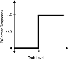
This figure shows that a person who has ability less than the value b has a 0% chance of getting the item correct. A person with trait level higher than b has a 100% chance of getting the item correct.

Of course, this is an unrealistic item, but it is illustrative in showing how a trait and a question probability relate to each other. More typical is a curve that allows probabilities that vary from zero to one. A typical curve found empirically is the S-shaped logistic function with a lower asymptote at zero and upper asymptote at one. It is markedly nonlinear. An example curve is shown in Figure 7.3.

The logistic model is the best choice to model this curve, because it has desirable asymptotic properties, yet is easier to deal with computationally than other proposed models (such as the cumulative normal density function). The model itself is

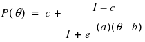
In this model, referred to as a Three-Parameter Logistic (3PL) model, the variable a represents the steepness of the curve at its inflection point. Curves with varying values of a are shown in Figure 7.4. This parameter can be interpreted as a measure of the discrimination of an item—that is, how much more difficult the item is for people with high levels of the trait than for those with low levels of the trait. Very large values of a make the model practically the step function shown in Figure 7.2. It is generally assumed that an examinee will have a higher probability of getting an item correct as their level of the trait increases. Therefore, a is assumed to be positive and the ICC is monotonically increasing. Some use this positive-increasing property of the curve as a test of the appropriateness of the item. Items whose curves do not have this shape should be considered as candidates to be dropped from the test.

Changing the value of b merely shifts the curve from left to right, as shown in Figure 7.5. It corresponds to the value of θ at the point where P(θ)=0.5. The parameter b can therefore be interpreted as item difficulty where (graphically), the more difficult items have their inflection points farther to the right along their x-coordinate.

Notice that

and therefore c represents the lower asymptote, which can be nonzero. ICCs for several values of c are shown graphically in Figure 7.6. The c parameter is theoretically pleasing, because a person with no ability of the trait might have a nonzero chance of getting an item right. Therefore, c is sometimes called the pseudo-guessing parameter.

By varying these three parameters, a wide variety of probability curves are available for modeling. A sample of three different ICCs is shown in Figure 7.7. Note that the lower asymptote varies, but the upper asymptote does not. This is because of the assumption that there might be a lower guessing parameter, but as the trait level increases, there is always a theoretical chance of 100% probability of correctly answering the item.

Note, however, that the 3PL model might by unnecessarily complex for many situations. If, for example, the c parameter is restricted to be zero (in practice, a reasonable restriction), there are fewer parameters to predict. This model, where only a and b parameters are estimated, is called the 2PL model.

Another advantage of the 2PL model (aside from its greater stability than the 3PL) is that b can be interpreted as the point where an examinee has a 50% chance of getting an item correct. This interpretation is not true for 3PL models.

A further restriction can be imposed on the general model when a researcher can assume that test items have equal discriminating power. In these cases, the parameter a is set equal to 1, leaving a single parameter to be estimated, the b parameter. This 1PL model is frequently called the Rasch model, named after Danish mathematician Georg Rasch, the developer of the model. The Rasch model is quite elegant, and is the least expensive to use computationally.

To launch the Item Analysis platform, select Analyze > Consumer Research > Item Analysis. This shows the dialog in Figure 7.8.

Specify the desired model (1PL, 2PL, or 3PL) by selecting it from the Model drop-down menu.

For this example, specify all fourteen continuous questions (Q1, Q2,..., Q14) as Y, Test Items and click OK. This accepts the default 2PL model.

If you select the 3PL model, a dialog pops up asking for a penalty for the c parameters (thresholds). This is not asking for the threshold itself. The penalty that it requests is similar to the type of penalty parameter that you would see in ridge regression, or in neural networks.

The penalty is on the sample variance of the estimated thresholds, so that large values of the penalty force the estimated thresholds’ values to be closer together. This has the effect of speeding up the computations, and reducing the variability of the threshold (at the expense of some bias).

In cases where the items are questions on a multiple choice test where there are the same number of possible responses for each question, there is often reason to believe (a priori) that the threshold parameters would be similar across items. For example, if you are analyzing the results of a 20-question multiple choice test where each question had four possible responses, it is reasonable to believe that the guessing, or threshold, parameters would all be near 0.25. So, in some cases, applying a penalty like this has some “physical intuition” to support it, in addition to its computational advantages.

Item characteristic curves for each question appear in the top section of the output. Initially, all curves are shown stacked in a single column. They can be rearranged using the Number of Plots Across command, found in the drop down menu of the report title bar. For Figure 7.9, four plots across are displayed.

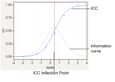
A vertical red line is drawn at the inflection point of each curve. In addition, dots are drawn at the actual proportion correct for each ability level, providing a graphical method of judging goodness-of-fit.

Gray information curves show the amount of information each question contributes to the overall information of the test. The information curve is the slope of the ICC curve, which is maximized at the inflection point.

Questions provide varying levels of information for different ability levels. The gray information curves for each item show the amount of information that each question contributes to the total information of the test. The total information of the test for the entire range of abilities is shown in the Information Plot section of the report (Figure 7.11).

The information gained from item difficulty parameters in IRT models can be used to construct an increasing scale of questions, from easiest to hardest, on the same scale as the examinees. This structure gives information about which items are associated with low levels of the trait, and which are associated with high levels of the trait.

JMP shows this correspondence with a dual plot. The dual plot for this example is shown in Figure 7.12.

Questions are plotted to the left of the vertical dotted line, examinees on the right. In addition, a histogram of ability levels is appended to the right side of the plot.

This example shows a wide range of abilities. Q10 is rated as difficult, with an examinee needing to be around half a standard deviation above the mean in order to have a 50% chance of correctly answering the question. Other questions are distributed at lower ability levels, with Q11 and Q4 appearing as easier. There are some questions that are off the displayed scale (Q7 and Q14).

The estimated parameter estimates appear below the Dual Plot, as shown in Figure 7.13.

An assumption of these IRT models is that the underlying trait is unidimensional. That is to say, there is a single underlying trait that the questions measure that can be theoretically measured on a continuum. This continuum is the horizontal axis in the plots of the curves. If there are several traits being measured, each of which have complex interactions with each other, then these unidimensional models are not appropriate.