
Example of Multiple Correspondence Analysis
This example uses the Car Poll.jmp sample data table, which contains data collected from car polls. The data include aspects about the individuals polled, such as sex, marital status, and age. The data also include aspects about the car that they own, such as the country of origin, the size, and the type. You want to explore relationships between sex, marital status, country and size of car to identify consumer preferences.
1. Select Help > Sample Data Library and open Car Poll.jmp.
2. Select Analyze > Consumer Research > Multiple Correspondence Analysis.
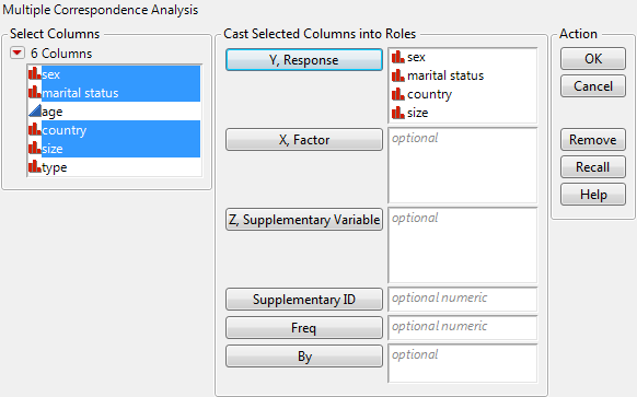
3. Select sex, marital status, country, and size and click Y, Response.
In MCA, usually all columns are considered responses rather than some being responses and others explanatory.
4. Click OK.
Figure 8.2 Completed Multiple Correspondence Analysis Launch Window
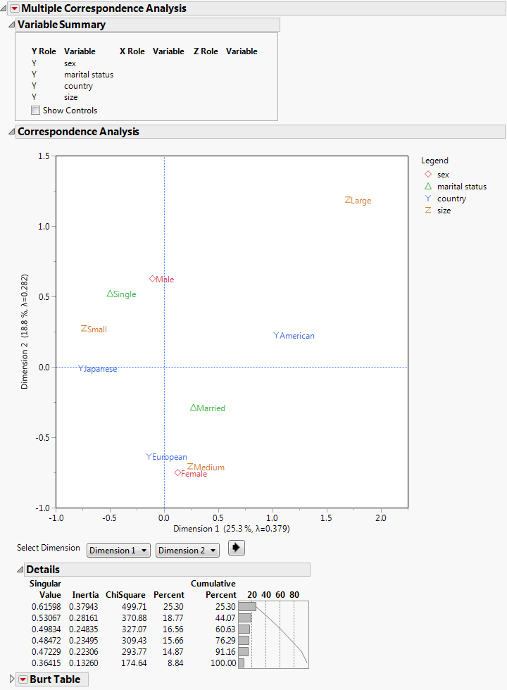
The Multiple Correspondence Analysis report is shown in Figure 8.3. Note that some of the outlines are closed because of space considerations.
The Variable Summary report provides a concise view of the analysis completed.
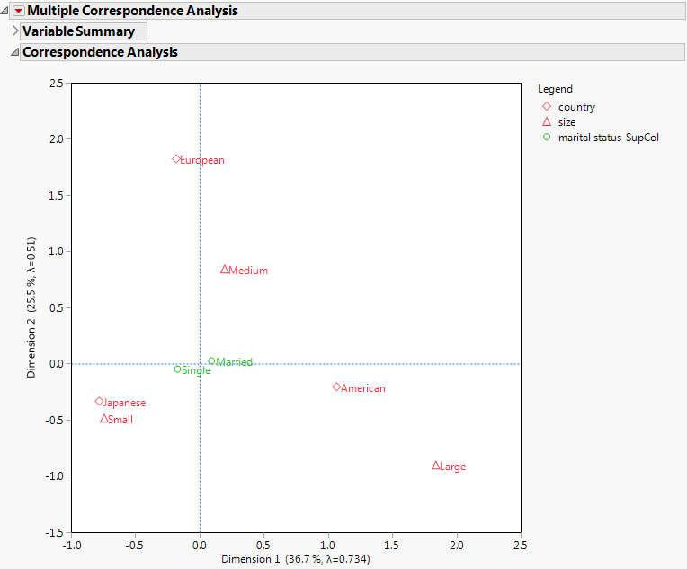
The Correspondence Analysis report shows the cloud of categories of the four variables as projected onto the two principal axes. From this cloud, you can see that Americans have a strong association with the large car size while Japanese are highly associated with the small car size. Also, males are strongly associated with the small car type and females are associated with the medium car size. This information could be used in market research to identify target audiences for advertisements.
Figure 8.3 Multiple Correspondence Analysis Report
Launch the Multiple Correspondence Analysis Platform
Launch the Multiple Correspondence Analysis platform by selecting Analyze > Consumer Research > Multiple Correspondence Analysis. This example uses the Car Poll.jmp sample data table.
Figure 8.4 Multiple Correspondence Analysis Launch Window
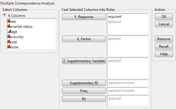
Y, Response
Assigns the categorical columns to be analyzed. Usually, in MCA, you are interested in the associations between variables, but there are not explicit “explanatory” and “response” variables.
X, Factor
Assigns the categorical columns to be used as factor, or explanatory, variables.
Z, Supplementary Variable
Assigns the columns to be used as supplementary variables. These variables are those you are interested in identifying associations with but not include in the calculations.
Supplementary ID
Assigns the column that identifies rows to be used as supplementary. A supplementary ID column usually has 1s and 0s. The rows associated with ID 0 are treated as supplementary rows. The Supplementary ID option functions if only one Y and only one X column have been specified.
Freq
Assigns a frequency variable to this role. This is useful if your data are summarized. In this instance, you have one column for the Y values and another column for the frequency of occurrence of the Y values.
By
Produces a separate report for each level of the By variable. If more than one By variable is assigned, a separate report is produced for each possible combination of the levels of the By variables.
The Multiple Correspondence Analysis Report
The initial Multiple Correspondence Analysis report shows the variable summary, correspondence analysis plot, and details of the dimensions of the data in order of importance. From the plot of the cloud of categories or individuals, you can identify associations that exist within the data. The details provide information about whether the two dimensions shown in the plot are sufficient to understand the relationships within the table.
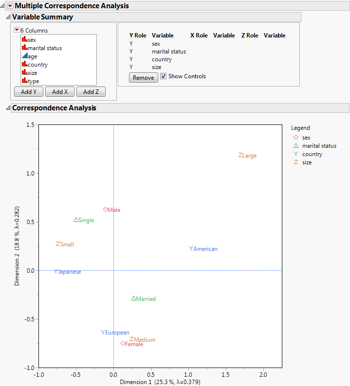
The Variable Summary shows the columns used in the analysis and the roles that you selected in the launch window. If you select the Show Controls check box, a list of the columns in the data table appears to the left. You can change the columns in the analysis either by selecting a column and clicking Add Y, Add X, or Add Z. Or you can drag the column to the header in the variable summary table. This enables you to modify the analysis without returning to the launch window.
Figure 8.5 Multiple Correspondence Analysis Report with Show Controls Selected
Multiple Correspondence Analysis Platform Options
The Multiple Correspondence Analysis red triangle menu options give you the ability to customize reports according to your needs. The reports available are determined by the type of analysis that you conduct.
Correspondence Analysis
Provides correspondence analysis reports. These reports give the plots, details, estimates of coordinates, and summary statistics. See “Additional Examples of the Multiple Correspondence Analysis Platform”.
Cross Table
Provides the Burt table or contingency table as appropriate for variable roles selected. See “Cross Table”.
Cross Table of Supplementary Rows
Provides a contingency table of the supplementary variable(s) versus the response variable(s). This table appears by default only if a supplementary variable has been specified in the launch window.
Cross Table of Supplementary Columns
Provides a contingency table of the X, Factor variable(s) versus the supplementary variable(s). This table appears by default only if a factor variable and a supplementary variable have been specified in the launch window.
Mosaic Plot
Displays a mosaic bar chart for each nominal or ordinal response variable. A mosaic plot is a stacked bar chart where each segment is proportional to its group’s frequency count. This option is available if only one Y and only one X variable are selected.
Tests for Independence
Provides the tests for independence whether there is association between the row and column variables. There are two versions of this test, the Pearson form and the Likelihood Ratio form, both with chi‐square statistics. This option is available only when there is one Y variable and one X variable.
Script
Contains options that are available to all platforms. See the Using JMP book.
Correspondence Analysis Options
The reports available under Correspondence Analysis are determined by the type of analysis that you conduct. Several of these reports are shown by default.
Show Plot
Shows the two-dimensional cloud of categories in the plane described by the first two principal axes. This plot appears by default.
Show Detail
Provides the details of the analysis including the singular values, inertias, ChiSquare statistics, percent, and cumulative percent. This report appears by default. See “Show Detail”.
Show Adjusted Inertia
Provides reports of the Benzecri and Greenacre adjusted inertia. See Benzecri (1979) and Greenacre (1984). This option is available only for MCA, that is all columns are Ys. See “Show Adjusted Inertia”.
Show Coordinates
Provides a report of up to the first three principal coordinates for the categories in the analysis, as appropriate. See “Show Coordinates”.
Show Summary Statistics
Provides a report of the summary statistics, Quality, Mass, and Inertia, for each category in the analysis. See “Show Summary Statistics”.
Show Partial Contributions to Inertia
Provides a report of the contribution of each category to the inertia for each of up to the first three dimensions. See “Show Partial Contributions to Inertia”.
Show Squared Cosines
Provides a report of the squared cosines of each category for each of up to the first three dimensions. See “Show Squared Cosines”.
3D Correspondence Analysis
Shows the three-dimensional cloud of categories of the Y, X, and Z variables in the space described by the first three principal axes. This option is not available if there are less than three dimensions.
Show Plot
The plot displays a projection of the cloud of categories or individuals onto the plane described by the first two principal axes. The distance scale is the same in all directions. You can toggle the dimensions shown in the plot using the Select Dimension controls below the plot. The first control defines the horizontal axis of the plot, and the second control defines the vertical axis of the plot. Click the arrow button to cycle through the dimensions shown in the plot.
Show Detail
Singular Value
Shows the singular value decomposition of the contingency table or Burt table. For the formula, see “Statistical Details for the Details Report”.
Inertia
Lists the square of the singular values, reflecting the relative variation accounted for in the canonical dimensions.
ChiSquare
Lists the portion of the overall Chi-square for the Burt or contingency table represented by the dimension.
Percent
Portion of inertia with respect to the total inertia.
Cumulative Percent
Shows the cumulative portion of inertia. If the first two singular values capture the bulk of the inertia, then the 2-D correspondence analysis plot is sufficient to show the relationships in the table.
Show Adjusted Inertia
The principal inertias of a Burt table in MCA are the eigenvalues. The problem with these inertias is that they provide a pessimistic indication of fit. Benzécri proposed an inertia adjustment. Greenacre argued that the Benzécri adjustment overestimates the quality of fit and proposed an alternate adjustment. Both adjustments are calculated for your reference. See “Statistical Details for Adjusted Inertia”.
Inertia
Lists the square of the singular values, reflecting the relative variation accounted for in the canonical dimensions.
Adjusted Inertia
Lists the adjusted inertia according to either the Benzécri or Greenacre adjustment.
Percent
Portion of adjusted inertia with respect to the total inertia.
Cumulative Percent
Shows the cumulative portion of adjusted inertia. If the first two singular values capture the bulk of the inertia, then the 2-D correspondence analysis plot is sufficient to show the relationships in the table.
Show Coordinates
Y
Lists the columns specified as Y, Response variables.
Category
Lists the levels of the Y variables.
Dimension 1, Dimension 2, Dimension 3
Lists the coordinate for the category along the respective principal axis. By default, the table shows the first three dimension columns. Additional dimension columns are hidden. To reveal these optional columns, right-click on the table and select the dimension columns from the Columns submenu.
If there are columns specified as X, Factor variables, the Coordinates report displays tables of both X and Y with the same report headings. If a Z, Supplementary Variable is specified, the coordinates are listed below the X and Y coordinates as applicable.
Show Summary Statistics
Y
Lists the columns specified as Y, Response variables.
Category
Lists the levels of the Y variables.
Quality
Lists the quality of the representation of the level by the solution.
Mass
Lists the row percentage from the Burt or contingency table.
Inertia
Lists the row marginal percentage of the total inertia accounted for by the respective point.
If there are columns specified as X, Factor variables, the Summary Statistics report displays tables of both X and Y with the same report headings. See “Statistical Details for Summary Statistics”.
Show Partial Contributions to Inertia
Y
Lists the columns specified as Y, Response variables.
Category
Lists the levels of the Y variables.
Dimension 1, Dimension 2, Dimension 3
Lists the contribution of the level to the inertia of the respective dimension. By default, the table shows the first three dimension columns. Additional dimension columns are hidden. To reveal these optional columns, right-click on the table and select the dimension columns from the Columns submenu.
Each category contributes to the inertia of each dimension. The partial contributions within each dimension sum to 1. If there are columns specified as X, Factor variables, the Partial Contributions to Inertia report displays tables of both X and Y with the same report headings. See “Statistical Details for Partial Contributions to Inertia”.
Show Squared Cosines
Y
Lists the columns specified as Y, Response variables.
Category
Lists the levels of the Y variables.
Dimension 1, Dimension 2, Dimension 3
Lists the quality of the representation of the level by the respective dimension. By default, the table shows the first three dimension columns. Additional dimension columns are hidden. To reveal these optional columns, right-click on the table and select the dimension columns from the Columns submenu.
The values indicate the quality of each point for the dimension listed. The squared cosine can be interpreted as the correlation of the point with the dimension. The sum of the squared cosines of the first two dimensions is equal to the quality indicated in the summary statistics report. The term refers to the fact that the value is also the squared cosine value of the angle the point makes with the dimension.
If there are columns specified as X, Factor variables, the Squared Cosines report displays tables of both X and Y with the same report headings.
Cross Table
The Burt table is the basis of the multiple correspondence analysis. It is a partitioned symmetric table of all pairs of categorical variables. The diagonal partitions are diagonal matrices (a cross-table of a variable with itself). The off-diagonal partitions are ordinary contingency tables. When you select multiple Y, Response columns with no X, Factor columns, the Burt table is created. If you select any X, Factor columns, a traditional contingency table is created instead of a Burt table.
The red triangle menu for the Burt or contingency table contains options of statistics to display in the table.
Count
Cell frequency, margin total frequencies, and grand total (total sample size). This appears by default.
Total %
Percent of cell counts and margin totals to the grand total. This appears by default.
Cell Chi Square
Chi-square values computed for each cell as (O - E)2 / E.
Col %
Percent of each cell count to its column total.
Row %
Percent of each cell count to its row total.
Expected
Expected frequency (E) of each cell under the assumption of independence. Computed as the product of the corresponding row total and column total divided by the grand total.
Deviation
Observed cell frequency (O) minus the expected cell frequency (E).
Col Cum
Cumulative column total.
Col Cum %
Cumulative column percentage.
Row Cum
Cumulative row total.
Row Cum %
Cumulative row percentage.
Make Into Data Table
Creates one data table for each statistic shown in the table.
Cross Table of Supplementary Rows
When a Z, Supplementary column is selected, a contingency table with the supplementary column levels as the rows and the response column levels as the columns is created. The red triangle menu contains the same options as the Burt Table.
Cross Table of Supplementary Columns
When an X, Factor column and a Z, Supplementary column are selected, a contingency table with the X, Factor levels as rows and the Supplementary levels as columns is created. The red triangle menu contains the same options as the Burt Table.
Additional Examples of the Multiple Correspondence Analysis Platform
Example Using a Supplementary Variable
This example uses the Car Poll.jmp sample data table, which contains data collected from car polls. The data include aspects about the individuals polled, such as sex, marital status, and age. The data also include aspects about the car that they own, such as the country of origin, the size, and the type. You want to explore relationships between sex, country, and size of car to identify consumer preferences.
1. Select Help > Sample Data Library and open Car Poll.jmp.
2. Select Analyze > Consumer Research > Multiple Correspondence Analysis.
3. Select country and size and click Y, Response.
4. Select marital status and click Z, Supplementary Variable.
5. Click OK.
Unlike in the first example, this analysis does not use marital status in the calculations. Marital status is plotted after the calculations are complete.
You see from the plot strong relationships between Japanese and Small cars as well as American and Large cars. The two marital statuses are plotted in a different color. Single people seem to prefer smaller cars a bit more than married people.
Figure 8.6 MCA with Supplementary Variable Report
Example Using a Supplementary ID
The United States census allows for examining population growth over the last century. The US Regional Population.jmp sample data table contains populations of the 50 US states grouped into regions for each of the census years from 1920 to 2010. Alaska and Hawaii are treated as supplementary regions because they were not states during the entire time, and they are not part of the contiguous United States. You are interested in whether the population growth in these two states differs from the rest of the US.
1. Select Help > Sample Data Library and open US Regional Population.jmp.
2. Select Analyze > Consumer Research > Multiple Correspondence Analysis.
3. Select Year and click Y, Response.
4. Select Region and click X, Factor.
5. Select ID and click Supplementary ID.
6. Select Population and click Freq.
7. Click OK.
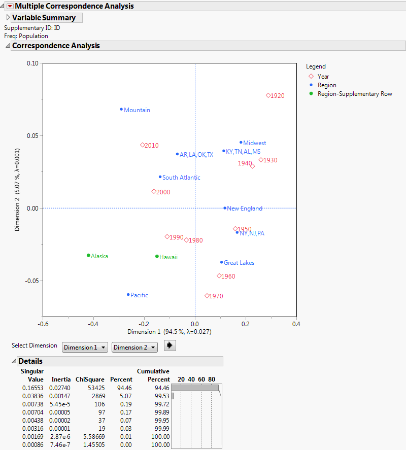
The Details report shows that the association between years and regions is almost entirely explained by the first dimension. The plot shows that years are in the correct order on the first dimension. This ordering occurs naturally through the correspondence analysis; there is no information about the order provided to the analysis.
Notice that the ordering of the regions reflects the population shift from the Midwest to the Northeast to the South and finally to the Mountain and West.
Alaska and Hawaii were not used in the computation of the analysis but are plotted based on the results. Their growth pattern is most similar to the Pacific states. Alaska’s growth is even more extreme than the Pacific region.
Figure 8.7 MCA with Supplementary ID Report
Statistical Details for the Multiple Correspondence Analysis Platform
Statistical Details for the Details Report
When a simple Correspondence Analysis is performed, the report lists the singular values of the following equation:
where:
• P is the matrix of counts divided by the total frequency
• r and c are row and column sums of P
• the Ds are diagonal matrices of the values of r and c
When Multiple Correspondence Analysis is performed, the singular value decomposition extends to:

where:

• C is the Burt table.
• Q is the number of categorical variables
• n is the number of observations
• 1 is a column vector of ones
Statistical Details for Adjusted Inertia
The usual principal inertias of a Burt table constructed from m categorical variables in MCA are the eigenvalues uk from  . These inertias provide a pessimistic indication of fit. Benzécri (1979) proposed the following inertia adjustment; it is also described by Greenacre (1984, p. 145):
 for
forThis adjustment computes the percent of adjusted inertia relative to the sum of the adjusted inertias for all inertias greater than  .
.
Greenacre (1994, p. 156) argues that the Benzécri adjustment overestimates the quality of fit. Greenacre proposes instead to compute the percentage of adjusted inertia relative to:

for all inertias greater than  , where
  is the sum of squared inertias and nc is the total number of categories across the m variables.
Statistical Details for Summary Statistics
Quality is the ratio of the sum of the squared cosines in the chosen number of dimensions and the sum of the squared cosines in the maximum number of dimensions. Quality indicates how well the point is represented in the reduced dimension space.
Inertia is the total Pearson Chi-square for a two-way frequency table divided by the sum of all observations in the table. In the summary statistics table, the relative inertia is listed.
Relative inertia is the proportion of the contribution of the point to the overall inertia.
Statistical Details for Partial Contributions to Inertia
The contribution of a row or column to the inertia of a dimension is calculated as:

..................Content has been hidden....................
You can't read the all page of ebook, please click here login for view all page.