
Choice Modeling Platform Overview
Choice modeling, pioneered by McFadden (1974), is a powerful analytic method used to estimate the probability of individuals making a particular choice from presented alternatives. Choice modeling is also called conjoint modeling, discrete choice analysis, and conditional logistic regression.
The Choice Modeling platform uses a form of conditional logistic regression. Unlike simple logistic regression, choice modeling uses a linear model to model choices based on response attributes and not solely upon subject characteristics. For example, in logistic regression, the response might be whether you buy brand A or brand B as a function of ten factors. The response could also be considered characteristics that describe you such as your age, gender, income, education, and so on. However, in choice modeling, you might be choosing between two cars that are a compound of ten attributes such as price, passenger load, number of cup holders, color, GPS device, gas mileage, anti-theft system, removable-seats, number of safety features, and insurance cost.
When engineers design a product, they routinely make hundreds or thousands of small design decisions. Most of these decisions are not tested by prospective customers. Consequently, these products are not optimally designed. However, if customer testing is not too costly and test subjects (prospective customers) are readily available, it is worthwhile to test more of these decisions via consumer choice experiments.
Modeling costs have recently decreased with improved product and process development techniques and methodologies. Prototyping, including pure digital prototyping, is becoming less expensive, so it is possible to evaluate the attributes and consequences of more alternatives. Another important advancement is the use of the Internet to deliver choice experiments to a wide audience. You can now inform your customers that they can have input into the design of the next product edition by completing a web survey.
Choice modeling can be added to Six Sigma programs to improve consumer products. Six Sigma aims at making products better by improving the manufacturing process and ensuring greater performance and durability. But, Six Sigma programs have not addressed one very important aspect of product improvement—making the products that people actually want. Six Sigma programs often consider the Voice of the Customer and can use customer satisfaction surveys. These surveys can disclose what is wrong with the product, but they fail to identify consumer preferences with regard to specific product attributes. Choice experiments provide a tool that enables companies to gain insight for actual customer preferences. Choice modeling analysis can reveal such preferences.
Market research experiments have a long history of success, but performing these experiments has been expensive, and research has previously focused on price elasticity and competitive situations. It is by using these same techniques for product design engineering where choice modeling can have the most impact.
Example of the Choice Platform
Suppose that you are supplying pizza for an airline. You want to find pizza attributes that are optimal for the flying population. So, you have a group of frequent flyers complete a choice survey. To weigh the importance of each attribute and potential interactions between attributes, you give them a series of choices that require them to state their preference between each pair of choices. One pair of choices might be between two types of pizza that they like, or between two types of pizza that they do not like. Hence, the choice might not always be easy.
This example examines pizza choices where three attributes, with two levels each, are presented to the subjects:
• crust (thick or thin)
• cheese (mozzarella or Monterey Jack)
• topping (pepperoni or none)
Suppose a subject likes thin crust with mozzarella cheese and no topping. The choices given to the subject are either a thick crust with mozzarella cheese and pepperoni topping, or a thin crust with Monterey Jack cheese and no topping. Because neither of these pizzas is ideal, the subject has to weigh which of the attributes are more important.
This example uses three data tables: Pizza Profiles.jmp, Pizza Responses.jmp, and Pizza Subjects.jmp.
1. Select Help > Sample Data Library and open Pizza Profiles.jmp, Pizza Responses.jmp, and Pizza Subjects.jmp.
The profile data table, Pizza Profiles.jmp, lists all the pizza choice combinations that you want to present to the subjects. Each choice combination is given an ID.
For the actual survey or experiment, each subject is given four trials, where each trial consists of stating his or her preference between two choice profiles (Choice1 and Choice2). The choice profiles given for each trial are referred to as a choice set. One subject’s choice trials can be different from another subject’s trials. Refer to the Discrete Choice Designs chapter in the Design of Experiments Guide. Notice that each choice value refers to an ID value in the Profile data table that has the attribute information.
Data about the subjects are stored in a separate Pizza Subjects.jmp file. This table includes a Subject ID column and characteristics of the subject. In the pizza example, the only characteristic or attribute about the Subject is Gender. Notice that the response choices and choice sets in the response data table use the ID names given in the Pizza Profiles.jmp data set. Similarly, the subject identifications in the response data table match those in the subject data table.
2. Select Analyze > Consumer Research > Choice to open the launch window.
There are three separate sections for each of the data sources.
3. Select Select Data Table under Profile Data.
A new window appears, which prompts you to specify the data table for the profile data.
4. Select Pizza Profiles.jmp.
The columns from this table now populate the field under Select Columns in the Choice Dialog box.
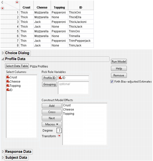
5. Select ID for Profile ID under Pick Role Variables and Add Crust, Cheese, and Topping under Construct Model Effects.
Figure 5.2 Profile Data Dialog
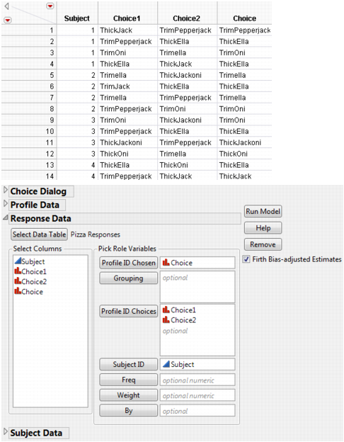
6. Open the Response Data section of the window. Click Select Data Table. When the Response Data Table window appears, select Pizza Responses.jmp.
7. Select Choice for the Profile ID Chosen, and Choice1 and Choice2 for the Profile ID Choices.
Figure 5.3 Response Data Dialog
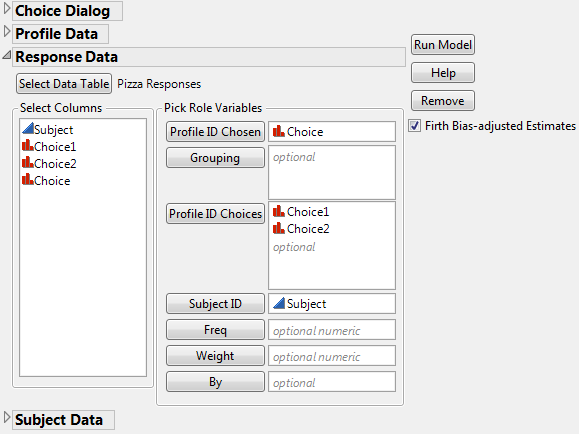
Choice1 and Choice2 are the profile ID choices given to a subject on each of four trials. The Choice column contains the chosen preference between Choice1 and Choice2.
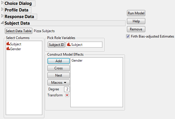
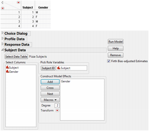
8. Open the Subject Data section of the window. Click Select Data Table. When the Subject Data Table window appears, select Pizza Subjects.jmp.
9. Select Subject for Subject ID to identify individual subjects.
10. Add Gender under Construct Model Effects.
Figure 5.4 Subject Data Dialog
11. Click Run Model.
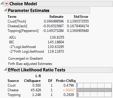
Figure 5.5 Choice Model Results
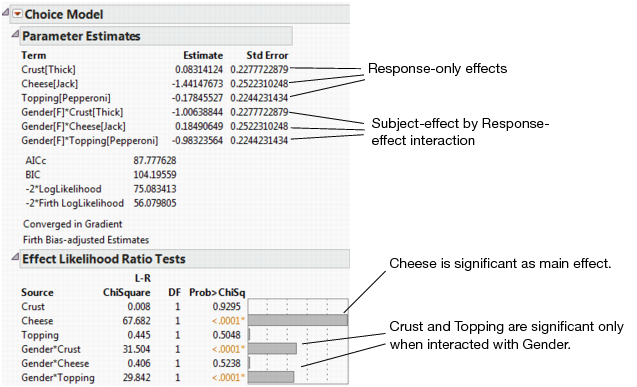
Figure 5.5 shows the parameter estimates and the likelihood ratio tests for the Choice Model with subject effects included. Strong interactions are seen between Gender and Crust and between Gender and Topping. When the Crust and Topping factors are assessed for the entire population, the effects are not significant. However, the effects of Crust and Topping are strong when they are evaluated between Gender groups.
Explore the Model
If you are concerned with selecting the best combination of factor levels, the Utility Profiler is a useful tool to explore and optimize your data.
1. From the Choice Model red triangle menu, select Utility Profiler.
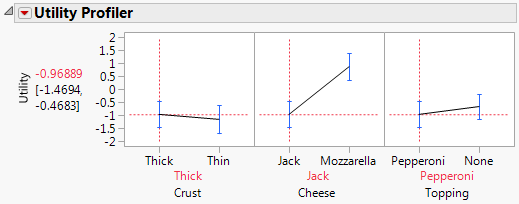
Figure 5.6 Utility Profiler with Female Level Factor Setting
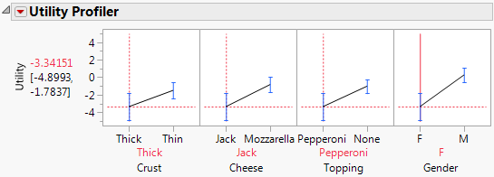
You can see that females do not particularly enjoy the default settings of thick crust with Jack cheese and pepperoni toppings.
2. Move the red line in the Gender plot to male (M).
Figure 5.7 Utility Profiler with Male Level Factor Setting

You can see that males prefer the default pizza more than females do, but not by much. To identify the optimal factor level settings, you must find their maximum desirability settings.
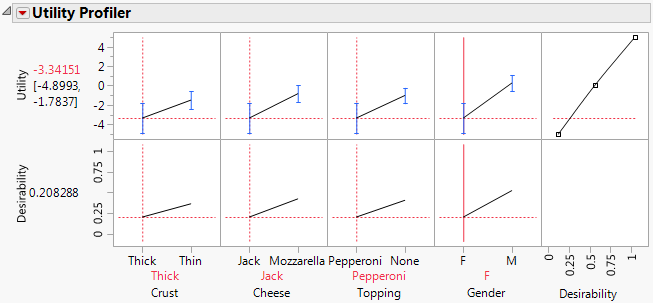
3. Click the red triangle menu of the Utility Profiler and select Desirability Functions.
A new row is added to the Utility Profiler, displaying overall desirability traces and measures. Utility and Desirability Functions are shown together in Figure 5.8.
Figure 5.8 Utility and Desirability Functions
4. From the red triangle menu of the Utility Profiler, select Maximize for each Grid Point.
A Remembered Settings table containing the grid settings with the maximum utility and desirability functions, and a table of differences between grids is displayed. See Figure 5.9. As illustrated, this feature can be a very quick and useful tool for selecting the most desirable attribute combinations for a factor.
Figure 5.9 Utility and Desirability Settings
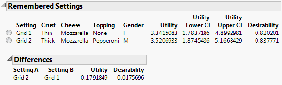
The grid setting for females shows that the greatest utility and desirability values are obtained when the pizza attributes are thin crust, mozzarella cheese, and no topping. For males, the grid setting shows that the highest utility and desirability values are obtained when the pizza attributes are thick crust, mozzarella cheese, and pepperoni topping. If you could offer two pizzas choices, these optimal settings for females and males would be the best to offer.
Launch the Choice Platform
Launch the Choice platform by selecting Analyze > Consumer Research > Choice.
The Choice platform is unique because it is designed to use data from one, two or three different data tables. Typically, data are in three separate tables: Profile Data, Response Data, and Subject Data. Each data table contains information that is joined together by the platform to extract the necessary data for Choice analysis. There are three sections of the Choice Launch Window. Each section corresponds to a different data table. If all your data are contained in one table, you can use the Choice platform, but additional effort is necessary. See the section “One-Table Analysis”.
Because the Choice platform can use several data tables, no initial assumption is made about using the current data table—as is the case with other JMP platforms. You must select the data table for each of the three choice data sources. You are prompted to select the profile data set and the response data set. If you want to model subject attributes, then a subject data set must also be selected. You can expand or collapse each section of the Choice window, as needed.
Profile Data
Profile data describe the attributes associated with each choice. Each choice can comprise many different attributes, and each attribute is listed as a column in the data table. There is a row for each possible choice, and each possible choice contains a unique ID. Figure 5.10 illustrates an example Profile Data table.
Figure 5.10 Example of Profile Data Table and Dialog Window
Select Data Table
Link to profile data table. You can select from any of the data sets already open in the current JMP session, or you can select Other. Selecting Other enables you to open a file that is not currently open.
Profile ID
Identifier for each row of choice combinations. If the Profile ID column does not uniquely identify each row in the profile data table, you need to add Grouping columns. Add Grouping columns until the combination of Grouping and Profile ID columns uniquely identify the row, or profile.
Grouping
With the Profile ID, unique identifier of each row, or profile. For example, if Profile ID = 1 for Survey = A, and a different Profile ID = 1 for Survey = B, then Survey would be used as a Grouping column.
For information about the Construct Model Effects window, see the Construct Model Effects section in the Introduction to Fit Model chapter of the Fitting Linear Models book.
Response Data
Response data contain the experimental results and have the choice set IDs for each trial as well as the actual choice selected by the subject. Each subject usually has several trials, or choice sets, to cover several choice possibilities. There can be more than one row of data for each subject. For example, an experiment might have 100 subjects with each subject making 12 choice decisions, resulting in 1200 rows in this data table. The Response data are linked to the Profile data through the choice set columns and the actual choice response column. Choice set refers to the set of alternatives from which the subject makes a choice. Grouping variables are sometimes used to align choice indices when more than one group is contained within the data.
Figure 5.11 Example of Response Data Table and Launch Window
Select Data Table
Link to response data table. You can select from any of the data sets already open in the current JMP session, or you can select Other. Selecting Other enables you to open a file that is not currently open.
Profile ID Chosen
The Profile ID from the Profile data table of the choice the subject selected.
Grouping
With the Profile ID Choices, unique identifier of each choice profile.
Profile ID Choices
The Profile IDs of the set of possible choices.
Subject ID
The Subject ID from the Subject data table.
Freq
The frequency of the observations. If n is the value of the Freq variable for a given row, then that row is used in computations n times. If it is less than 1 or missing, then JMP does not use it to calculate any analyses.
Weight
The weights for each observation in the data table. The variable does not have to be an integer, but it is included only in analyses when its value is greater than zero.
By
Levels in the data to create separate analyses.
Subject Data
Subject data are optional, depending on whether subject effects are to be modeled. This source contains one or more attributes or characteristics of each subject and a subject identifier. The Subject data table contains the same number of rows as subjects and has an identifier column that matches a similar column in the Response data table. You can also put Subject data in the Response data table, but it is still specified as a subject table.
Figure 5.12 Example of Subject Data Table and Launch Window
Select Data Table
Link to subject data table. You can select from any of the data sets already open in the current JMP session, or you can select Other. Selecting Other enables you to open a file that is not currently open.
Subject ID
Unique identifier of the subject.
For information about the Construct Model Effects window, see the Construct Model Effects section in the Introduction to Fit Model chapter of the Fitting Linear Models book.
Scripting the Choice Platform
If you are scripting the Choice platform, you can also set the acceptable criterion for convergence when estimating the parameters by adding this command to the Choice() specification:
Choice( ..., Convergence Criterion( fraction ), ... )
See the JMP Scripting Index in the Help menu for an example.
Choice Model Output
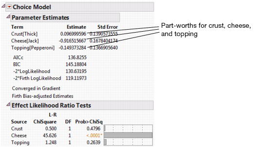
An example of the Choice Model Output results is shown in Figure 5.13.
• The resulting parameter estimates are sometimes referred to as part-worths. Each part-worth is the coefficient of utility associated with that attribute. By default, these estimates are based on the Firth bias-corrected maximum likelihood estimators and therefore are considered to be more accurate than MLEs without bias correction.
• Comparison criteria are used to help determine the better-fitting model(s) when more than one model is investigated for your data. The model with the lower or lowest criterion value is believed to be the better or best model. Criteria are shown in the Choice Model output and include AICc (corrected Akaike’s Information Criterion), BIC (Bayesian Information Criterion), − 2 LogLikelihood, and − 2 Firth Loglikelihood. The AICc formula is:
where k is the number of estimated parameters in the model and n is the number of observations in the data set. The BIC formula is: − 2 LogLikelihood + k ∗ ln(n), where k parameters is fitted to data with n observations and LogLikelihood is the maximized log-likelihood. Note that the − 2 Firth Loglikelihood result is included only in the report when the Firth Bias-adjusted Estimates check box is checked in the launch window. (See Figure 5.10.) This option is checked by default. The decision to use or not use the Firth Bias-adjusted Estimates does not affect the AICc score or the − 2 LogLikelihood results.
• Likelihood ratio tests appear for each effect in the model. These results are obtained by default if the model is fit quickly (less than five seconds). Otherwise, you can select the Choice Model red triangle menu and select Likelihood Ratio Tests.
Figure 5.13 Choice Model Results with No Subject Data for Pizza Example
Choice Platform Options
The Choice Modeling platform has many available options. To access these options, select the Choice Model red triangle menu.
Likelihood Ratio Tests
Tests the significance of each effect in the model. These are done by default if the estimate of CPU time is less than five seconds.
Joint Factor Tests
Tests each factor in the model by constructing a likelihood ratio test for all the effects involving that factor. For more information about Joint Factor Tests, see the Standard Least Squares Report and Options chapter of the Fitting Linear Models.
Confidence Intervals
Produces a 95% confidence interval for each parameter (by default), using the profile-likelihood method. Shift-click the platform red triangle menu and select Confidence Intervals to input alpha values other than 0.05.
Correlation of Estimates
Shows the correlations of the parameter estimates.
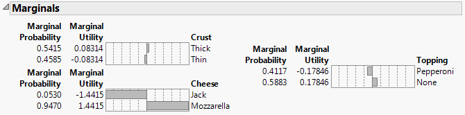
Effect Marginals
Shows the fitted utility values for different levels in the effects, with neutral values used for unrelated factors. Effect Marginals also includes marginal probabilities. The marginal probability is the probability of an individual selecting attribute factor A over factor B with all other attributes at their mean or default levels. For example, the marginal probability of any subject choosing a pizza with mozzarella cheese, thick crust and pepperoni over that same pizza with Monterey Jack cheese instead of mozzarella is 0.9470.
Figure 5.14 Example of Marginal Effects
Utility Profiler
Shows the predicted utility for different factor settings. The utility is the value predicted by the linear model. See “Explore the Model” for an example of the Utility Profiler. For details about the Utility Profiler options, see the Prediction Profiler Options section in the Profiler chapter of the Profilers book.
Probability Profiler
Shows the predicted probability for choosing the given factor settings compared with baseline factor settings. This predicted probability is defined as  , where U is the utility for the current settings and Ub is the utility for the baseline settings. See “Compare to Baseline” for an example of using the Probability Profiler. For details about the Probability Profiler options, see the Prediction Profiler Options section in the Profiler chapter of the Profilers book.
Multiple Choice Profiler
Enables you to set up a number of choice sets and see the probabilities of choosing each set relative to the other choices. See “Multiple Choice Comparison” for an example of using the Multiple Choice Profiler. For details about the Multiple Choice Profiler options, see the Prediction Profiler Options section in the Profiler chapter of the Profilers book.
Comparisons
Performs comparisons between specific alternative choice profiles. Enables you to select factor values and the values that you want to compare. From here you can compare specific configurations, including comparing all settings on the left or right by selecting the Any check boxes. Using Any does not compare all combinations across features, but rather all combinations of comparisons, one feature at a time, using the left settings as the settings for the other factors.
Figure 5.15 Comparisons Example
Willingness to Pay
Calculates how much a price must change allowing for the new feature settings to produce the same predicted outcome. The result is calculated using the Baseline settings (for each background setting) and then determining the outcome after altering the Role, including.
‒ Feature Factor - a feature in the experiment that you want to price.
‒ Price Factor - a continuous price factor in the experiment.
‒ Background Constant - something that you want to hold constant at a baseline value.
‒ Background Variable - something that you want to iterate across values.
Figure 5.16 Willingness to Pay Example
The Include baseline settings in report table option adds the baseline settings with a price change of zero, which is useful if you make an output table of these prices displaying all the baseline settings as well as the featured settings.
Save Utility Formula
Makes a new column with a formula for the utility, or linear model, that is estimated. This is in the profile data table, except if there are subject effects. In that case, it makes a new data table for the formula. This formula can be used with various profilers with subsequent analyses. For more details about the Utility Formula, see “Statistical Details”.
Save Gradients by Subject
Constructs a new table that has a row for each subject containing the average (Hessian-scaled-gradient) steps on each parameter. This corresponds to using a Lagrangian multiplier test for separating that subject from the remaining subjects. These values can later be clustered, using the built-in-script, to indicate unique market segments represented in the data. For more details, see “Segmentation”.
Model Dialog
Shows the Choice launch window, which can be used to modify and re-fit the model. You can specify new data sets, new IDs, and new model effects.
Valuing Trade-offs
The Choice Modeling platform is also useful for determining the relative importance of product attributes. Even if the attributes of a particular product that are important to the consumer are known, information about preference trade-offs with regard to these attributes might be unknown. By gaining such information, a market researcher or product designer is able to incorporate product features that represent the optimal trade-off from the perspective of the consumer. The advantages of this approach to product design can be found in the following example.
Example of Valuing Trade-offs
It is already known that four attributes are important for laptop design: hard-disk size, processor speed, battery life, and selling price. The data gathered for this study are used to determine which of four laptop attributes (Hard Disk, Speed, Battery Life, and Price) are most important. It also assesses whether there are Gender or Job differences seen with these attributes.
1. Select Help > Sample Data Library and open Laptop Profile.jmp.
2. Select Analyze > Consumer Research > Choice to open the launch window.
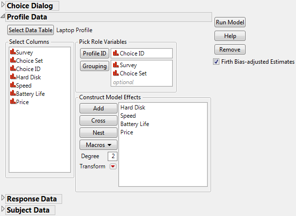
3. Click Select Data Table under Profile Data and select Laptop Profile.jmp. A partial listing of the Profile Data table is shown in Figure 5.17. The complete data set consists of 24 rows, 12 for Survey 1 and 12 for Survey 2. Survey and Choice Set define the grouping columns and Choice ID represents the four attributes of laptops: Hard Disk, Speed, Battery Life, and Price.
Figure 5.17 Profile Data Set for the Laptop Example
4. Select Choice ID for Profile ID, and Add Hard Disk, Speed, Battery Life, and Price for the model effects.
5. Select Survey and Choice Set as the Grouping columns. The Profile Data window is shown in Figure 5.18.
Figure 5.18 Profile Data Dialog Box for Laptop Study
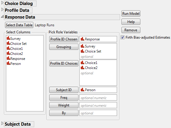
6. Click Response Data > Select Data Table > Other > OK and select Laptop Runs.jmp from the sample data library.
7. Select Response as the Profile ID Chosen, Choice1, and Choice2 as the Profile ID Choices, Survey and Choice Set as the Grouping columns, and Person as Subject ID. The Response Data window is shown in Figure 5.19.
Figure 5.19 Response Data Dialog Box for Laptop Study
8. To run the model without subject effects, click Run Model.
9. Choose Utility Profiler from the red triangle menu.
Figure 5.20 Laptop Results without Subject Effects
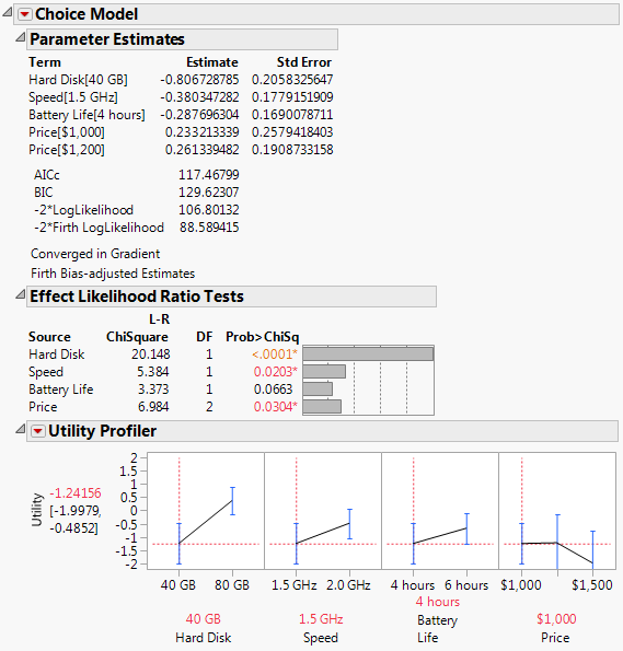
Results of this study show that while all the factors are important, the most important factor in the laptop study is Hard Disk. The respondents prefer the larger size. Note that respondents did not think a price increase from $1000 to $1200 was important, but an increase from $1200 to $1500 was considered important. This effect is easily visualized by examining the factors interactively with the Utility Profiler. Such a finding can have implications for pricing policies, depending on external market forces.
Subject Effects
To include subject effect for the laptop study, simply add to the Choice Modeling window.
1. Select Model Dialog from the Choice Model red triangle menu.
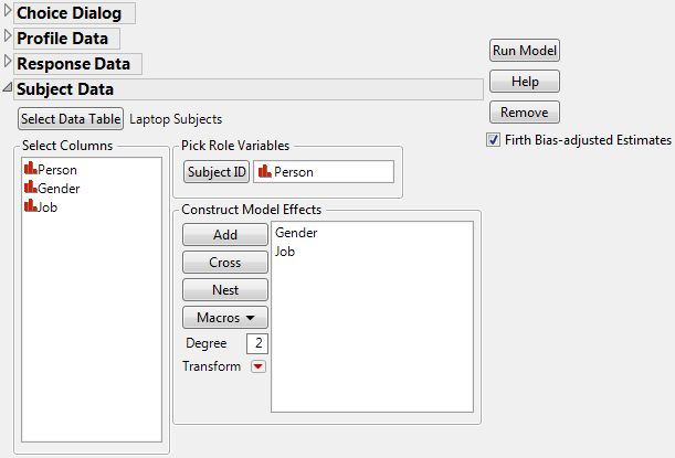
2. Under Subject Data, Select Data Table > Other > OK > Laptop Subjects.jmp.
3. Select Person as Subject ID and Add Gender and Job as the model effects.
The Subject Data window is shown in Figure 5.21.
Figure 5.21 Subject Dialog Box for Laptop Study
4. Click Run Model.
Figure 5.22 Laptop Parameter Estimate Results with Subject Data
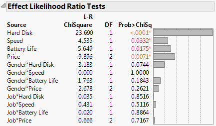
Figure 5.23 Laptop Likelihood Ratio Test Results with Subject Data
5. Select Joint Factor Tests from the Choice Model red triangle menu
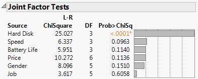
The results of the Joint Factor Tests are displayed in Figure 5.24.
Figure 5.24 Joint Factor Test for Laptop
6. Select Effect Marginals from the Choice Model red triangle menu.
The marginal effects of each level for each factor are displayed in Figure 5.25. Notice that the marginal effects for each factor across all levels sum to zero.
Figure 5.25 Marginal Effects for Laptop
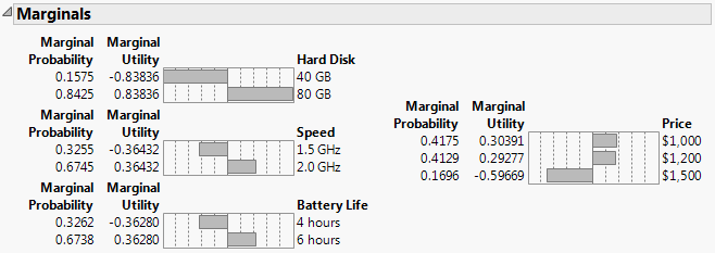
Figure 5.26 Laptop Profiler Results for Females with Subject Data
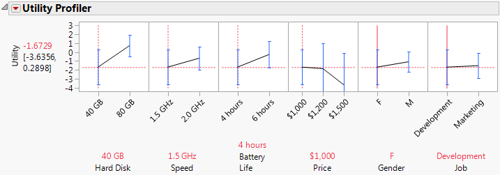
Figure 5.27 Laptop Profiler Results for Males with Subject Data
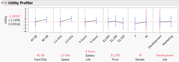
The interaction effect between Gender and Hard Disk is marginally significant, with a p-value of 0.0744 (See Figure 5.23). In the Utility Profiler, check the slope for Hard Disk for both levels of Gender. You see that the slope is steeper for females than for males.
Compare to Baseline
If you wanted to know the probability of a customer selecting one choice over some baseline, the Probability Profiler is useful to compare choices. Suppose you were developing a new product and wanted to see the likelihood of a customer selecting the new product over the old product or a competitor’s product. The Probability Profiler is a useful tool for this type of baseline analysis.
In this example, your company is currently producing laptops with 40 GB hard drives, 1.5 GHz processors, and 6 hour battery life that costs $1,200. You are looking for a way to make your product more desirable by changing as few factors as possible.
1. From the Choice Model red triangle window, select Probability Profiler.
2. Set the Baseline to 40 GB, 1.5 GHz, 6 hours, and $1,200.
3. In the Probability Profiler, change the settings of Battery Life to 6 hours and Price to $1,200.
Figure 5.28 Laptop Probability Profiler Results with Baseline Effects
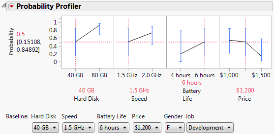
You can see in Figure 5.28 that by increasing Hard Disk space, increasing Speed, or decreasing the price would increase the probability a subject would choose the new product over the old for females with development jobs.
4. Change the Gender effect in the Baseline to M.
You can see that by decreasing price, males with development jobs are actually less likely to choose the new product over the old. If you change the Job effect in the Baseline to Marketing, you see the same effect.
Looking at Figure 5.28, you can see that the steepest slope is for the Hard Disk factor.
5. Change the Gender Effect in the Baseline to F and change the Hard Disk to 80 GB in the Probability Profiler.
Figure 5.29 Laptop Probability Profiler Results with More Space
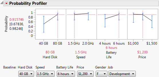
By increasing the space in the new laptop, a female with a development job choose the new laptop over the old laptop almost 92% of the time.
You can change the subject effects to vary gender and job. The probability results are displayed in Table 5.1. You can see that males in development jobs are less likely than females in the same job to choose the new laptop, they are still more likely to choose the new laptop over the old. Developing a new product with increased hard disk space is more desirable to your customers than the old product.
|
Gender
|
Job
|
Probability of Selecting New Laptop over Old
|
|
Female
|
Development
|
0.915746
|
|
Female
|
Marketing
|
0.938172
|
|
Male
|
Development
|
0.696043
|
|
Male
|
Marketing
|
0.761733
|
Multiple Choice Comparison
If, for example, you wanted to develop a product that had an advantage over two other competitors, you could use the Multiple Choice Profiler. The Multiple Choice Profiler enables you to determine the probability of a subject choosing one choice set over various others.
Company A produces a product with a fast processor speed and high battery life at a reasonable price. Company B makes the biggest hard drives with the fastest speed, but at a high price and low battery life. You currently make a low-end laptop with small hard drive, slow processor, and low battery life. You want to gain market share by increasing one area of performance and price.
You want to market this product to the masses, so you want to remove the subject effects.
1. From the Choice Model red triangle window, select Model Dialog.
2. Open the Subject Data section. Click Subject Data Table.
The Subject DataTable window appears, prompting you to select a data table to use.
3. Ensure that no data table is selected and click OK. By default, no data table is selected.
4. Click Run Model.
5. From the Choice Model red triangle window, select Multiple Choice Profiler.
A window appears, asking for the number of alternative choices to profile. The default number 3 is already entered in the window.
6. Click OK.
Three Alternative profilers appear. Each factor in each profiler is set to their default values. Alternative 1 indicates the product that you want to develop. Alternative 2 indicates Company A’s product. Alternative 3 indicates Company B’s product.
7. For Alternative 2, set Hard Disk to 40 GB, Speed to 2.0 GHz, Battery Life to 6 hours, and Price to $1,200.
8. For Alternative 3, set Hard Disk to 80 GB, Speed to 2.0 GHz, Battery Life to 4 hours, and Price to $1,500.
Figure 5.30 Multiple Choice Profiler with Laptop Data
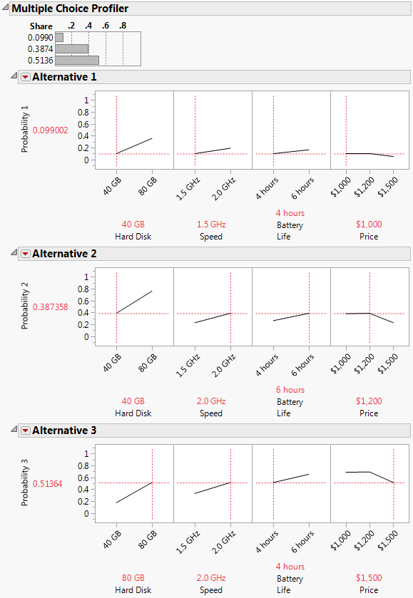
You can see that with your company’s settings set to the low, default levels, Company B has the greatest Share of 0.51364. This Share means that the probability of any subject choosing Alternative 3 is 51.4%. It is obvious that with your company’s settings set how they are, very few people buy your product.
You want to increase your market share by upgrading your company’s laptop in one of the performance areas and increasing price. The slope of the line in Alternative 1’s Hard Disk profile suggests increasing hard disk space will increase market share the most.
9. For Alternative, set Hard Disk to 80 GB and Price to $1,200.
Figure 5.31 Multiple Choice Profiler with Improved Laptop
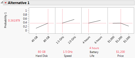
By increasing hard disk space, you can increase the price of your laptop and expect a market share of about 36%. This share is almost the same as Company B’s high-performance laptop and is much better than the market share with the initial low-end settings seen in Figure 5.30.
You can see in Figure 5.31 that you could increase your market share even more by increasing Speed or Battery Life. If you wanted to determine what laptop configuration would give you the maximum market share, you could maximize desirability using the Choice Model red triangle menu options. In this case, however, it is fairly obvious that a high-performance laptop at a low price would be the most desirable.
One-Table Analysis
The Choice Modeling platform can also be used if all of your data are in one table. For this one-table scenario, you use only the Profile Data section of the Choice Dialog box. Subject-specific terms can be used in the model, but not as main effects. Two advantages, both offering more model-effect flexibility than the three-table specification, are realized by using a one-table analysis:
• Interactions can be selectively chosen instead of automatically getting all possible interactions between subject and profile effects as seen when using three tables.
• Unusual combinations of choice sets are allowed. This means, for example, that the first trial can have a choice set of two, the second trial can consist of a choice set of three, the third trial can have a choice set of five, and so on. With multiple tables, in contrast, it is assumed that the number of choices for each trial is fixed.
A choice response consists of a set of rows, uniquely identified by the Grouping columns. An indicator column is specified for Profile ID in the Choice Dialog box. This indicator variable uses the value of 1 for the chosen profile row and 0 elsewhere. There must be exactly one “1” for each Grouping combination.
Example of One-Table Analysis
This example illustrates how the pizza data are organized for the one-table situation. Figure 5.32 shows a subset of the combined pizza data.
1. Select Help > Sample Data Library and open Pizza Combined.jmp to see the complete table.
Each subject completes four choice sets, with each choice set or trial consisting of two choices. For this example, each subject has eight rows in the data set. The indicator variable specifies the chosen profile for each choice set. The columns Subject and Trial together identify the choice set, so they are the Grouping columns.
Figure 5.32 Partial Listing of Combined Pizza Data for One-Table Analysis
To analyze the data in this format, open the Profile Data section in the Choice Dialog box, shown in Figure 5.33.
2. Select Analyze > Consumer Research > Choice.
3. Click Select Data Table.
4. Specify Pizza Combined.jmp as the data set. Click OK.
5. In the Profile Data section of the window, specify Indicator as the Profile ID, Subject and Trial as the Grouping variables, and add Crust, Cheese, and Topping as the main effects.
See Figure 5.33.
Figure 5.33 Choice Dialog Box for Pizza Data One-Table Analysis
6. Click Run Model.
A new window appears, asking if this is a one-table analysis with all of the data in the Profile Table.
7. Click Yes to fit the model, as shown in Figure 5.34.
Figure 5.34 Choice Model for Pizza Data One-Table Analysis
8. Select Utility Profiler from the drop-down menu to obtain the results shown in Figure 5.35. Notice that the parameter estimates and the likelihood ratio test results are identical to the results obtained for the Choice Model with only two tables, shown in Figure 5.13.
Figure 5.35 Utility Profiler for Pizza Data One-Table Analysis
Segmentation
Market researchers sometimes want to analyze the preference structure for each subject separately in order to see whether there are groups of subjects that behave differently. However, there are usually not enough data to do this with ordinary estimates. If there are sufficient data, you can specify “By groups” in the Response Data or you could introduce a Subject identifier as a subject-side model term. This approach, however, is costly if the number of subjects is large. Other segmentation techniques discussed in the literature include Bayesian and mixture methods.
You can also use JMP to segment by clustering subjects using response data. For example, after running the model using the Pizza Profiles.jmp, Pizza Responses.jmp, and the optional Pizza Subjects.jmp data sets, select the red triangle menu for the Choice Model platform and select Save Gradients by Subject. A new data table is created containing the average Hessian-scaled gradient on each parameter, and there is one row for each subject.
Note: This feature is regarded as an experimental method, because, in practice, little research has been conducted on its effectiveness.
These gradient values are the subject-aggregated Newton-Raphson steps from the optimization used to produce the estimates. At the estimates, the total gradient is zero, and Δ = H-1g = 0, where g is the total gradient of the log-likelihood evaluated at the MLE, and H-1 is the inverse Hessian function or the inverse of the negative of the second partial derivative of the log-likelihood.
But, the disaggregation of Δ results in
Δ = ΣijΔij = ΣH-1gij = 0,
where i is the subject index, j is the choice response index for each subject, Δij are the partial Newton-Raphson steps for each run, and gij is the gradient of the log-likelihood by run.
The mean gradient step for each subject is then calculated as:
 ,
,where ni is the number of runs per subject. These Δi are related to the force that subject i is applying to the parameters. If groups of subjects have truly different preference structures, these forces are strong, and they can be used to cluster the subjects. The Δi are the gradient forces that are saved. You can then cluster these values using the Clustering platform.
Example of Segmentation
Set Up the Model
1. Select Help > Sample Data Library and open Pizza Profiles.jmp, Pizza Responses.jmp, and Pizza Subjects.jmp.
2. Select Analyze > Consumer Research > Choice to open the launch window.
There are three separate sections for each of the data sources.
3. Select Select Data Table under Profile Data.
You are prompted to select the data table for the profile data.
4. Select Pizza Profiles.jmp.
The columns from this table now populate the field under Select Columns in the Choice Dialog box.
5. Select ID and click Profile ID.
6. Select Crust, Cheese, and Topping and click Add.
7. Open the Response Data section of the window and click Select Data Table.
8. Select Pizza Responses.jmp.
9. Select Choice and click Profile ID Chosen
10. Select Choice1 and Choice2 and click Profile ID Choices.
11. Select Subject and click Subject ID.
12. Open the Subject Data section of the window and click Select Data Table.
13. Select Pizza Subjects.jmp.
14. Select Subject and click Subject ID to identify individual subjects.
15. Select Gender and click Add.
16. Click Run Model.
The Choice Model report appears.
Cluster Subjects
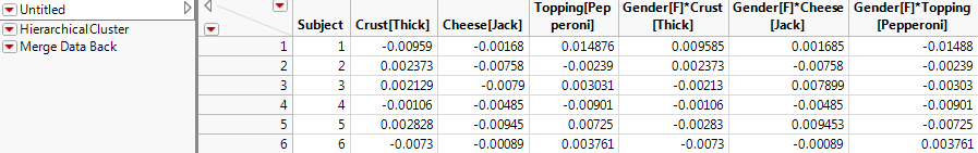
1. In the Choice Model red triangle menu, select Save Gradients by Subject.
A new data table is generated, with gradient forces saved for each main effect and subject interaction. A partial data table with these subject gradient forces is shown in Figure 5.36.
Figure 5.36 Gradients by Subject for Pizza Data
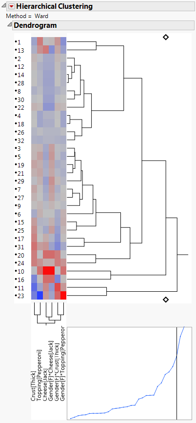
2. In the new data table, click the red triangle menu of the HierarchicalCluster script. Click Run Script.
The resulting dendrogram of the clusters is shown in Figure 5.37.
Figure 5.37 Dendrogram of Subject Clusters for Pizza Data
3. Save the cluster IDs by clicking on the red triangle menu of Hierarchical Clustering and selecting Save Clusters.
A new column called Cluster is created in the data table containing the gradients. Each subject has been assigned a Cluster value that is associated with other subjects having similar gradient forces. Refer to the Cluster platform chapter in the Multivariate Methods book for a discussion of other Hierarchical Clustering options. The gradient columns can be deleted because they were used only to obtain the clusters.
4. Select all columns except Subject and Cluster. Right-click on the selected columns and select Delete Columns.
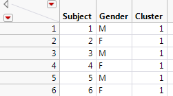
The data table shown in Figure 5.38 contains only Subject and Cluster variables.
Figure 5.38 Merge Results Back into Original Table
5. Click Run Script under the Merge Data Back red triangle menu, as shown in the partial gradient-by-subject table in Figure 5.36.
The cluster information is merged into the Subject data table.
The columns in the Subject data table are now Subject, Gender, and Cluster, as shown in Figure 5.39.
Figure 5.39 Subject Data with Cluster Column
This table can then be used for further analysis.
Fit Y by X
1. Select Analyze > Fit Y by X.
2. Specify Gender as the Y, Response, and Cluster as X, Factor.
This analysis is depicted in Figure 5.40.
Figure 5.40 Contingency Analysis of Gender by Cluster for Pizza Example
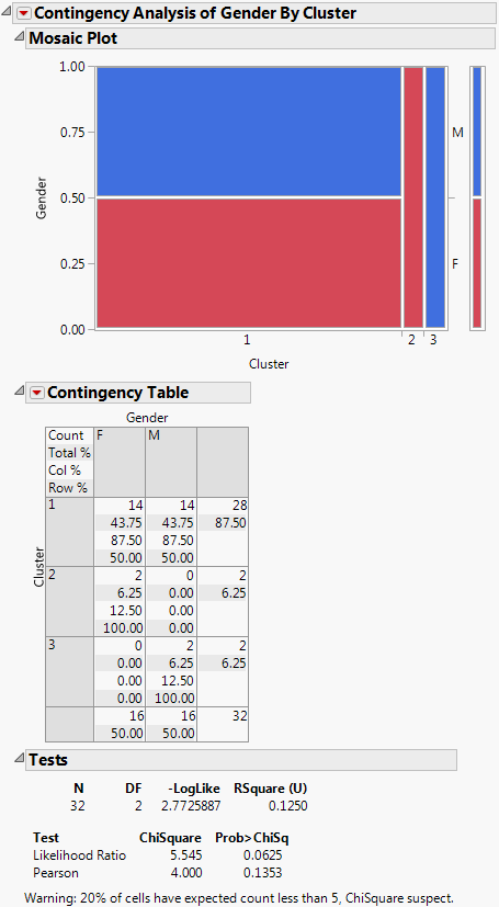
Figure 5.40 shows that Cluster 1 contains half male and female, Cluster 2 is only female, and Cluster 3 is all male. If desired, you could now refit and analyze the model with the addition of the Cluster variable.
Special Data Rules
Default Choice Set
If in every trial, you can choose any of the response profiles, you can omit the Profile ID Choices selection under Pick Role Variables in the Response Data section of the Choice Dialog Box. The Choice Model platform then assumes that all choice profiles are available on each run.
Subject Data with Response Data
If you have subject data in the Response data table, select this table as the Select Data Table under the Subject Data. In this case, a Subject ID column does not need to be specified. In fact, it is not used. It is generally assumed that the subject data repeats consistently in multiple runs for each subject.
Logistic Regression
Ordinary logistic regression can be done with the Choice Modeling platform.
Note: The Fit Y by X and Fit Model platforms are more convenient to use than the Choice Modeling platform for logistic regression modeling. This section is used only to demonstrate that the Choice Modeling platform can be used for logistic regression, if desired.
If your data are already in the choice-model format, you might want to use the steps given below for logistic regression analysis. However, three steps are needed:
• Create a trivial Profile data table with a row for each response level.
• Put the explanatory variables into the Response data.
• Specify the Response data table, again, for the Subject data table.
For examples of conducting Logistic Regression using the Choice Platform, see“Example of Logistic Regression Using the Choice Platform” and “Example of Logistic Regression for Matched Case-Control Studies”.
Transforming Data
Although data are often in the Response/Profile/Subject form, the data are sometimes specified in another format that must be manipulated into the normalized form needed for choice analysis.
Example of Transforming Data to Two Analysis Tables
Consider the data from Daganzo, found in Daganzo Trip.jmp. This data set contains the travel time for three transportation alternatives and the preferred transportation alternative for each subject.
Add Choice Mode and Subjects
1. Select Help > Sample Data Library and open the Daganzo.jmp data table.
A partial listing of the data set is shown in Figure 5.41.
Figure 5.41 Partial Daganzo Travel Time Table for Three Alternatives
Each Choice number listed must first be converted to one of the travel mode names. This transformation is easily done by using the Choose function in the formula editor, as follows.
2. Select Cols > New Column.
3. Specify the Column Name as Choice Mode and the modeling type as Nominal.
4. Click the Column Properties and select Formula.
5. Click Conditional under the Functions (grouped) command, select Choose, and press the comma key twice to obtain additional arguments for the function.
6. Click Choice for the Choose expression (expr), and double click each clause entry box to enter “Subway”, “Bus”, and “Car” (with the quotation marks) as shown in Figure 5.42.
Figure 5.42 Choose Function for Choice Mode Column of Daganzo Data
7. Click OK in the Formula Editor window.
8. Click OK in the New Column window.
The new Choice Mode column appears in the data table. Because each row contains a choice made by each subject, another column containing a sequence of numbers should be created to identify the subjects.
9. Select Cols > New Column.
10. Specify the Column Name as Subject.
11. Click Missing/Empty next to Initialize Data and select Sequence Data.
12. Click OK.
A partial listing of the modified table is shown in Figure 5.43.
Figure 5.43 Daganzo Data with New Choice Mode and Subject Columns
Stack the Data
In order to construct the Profile data, each alternative needs to be expressed in a separate row.
1. Selecting Tables > Stack.
2. Select the columns Subway, Bus, and Car and click Stack Columns.
3. For the Output table name, type Stacked Daganzo. Type Travel Time for the Stacked Data Column and Mode for the Source Label Column.
The resulting Stack window is shown in Figure 5.44.
Figure 5.44 Stack Operation for Daganzo Data
4. Click OK.
A partial view of the resulting table is shown in Figure 5.45.
Figure 5.45 Partial Stacked Daganzo Table
Make the Profile Data Table
For the Profile Data Table, you need the Subject, Mode, and Travel Time columns.
1. Select the Subject, Mode, and Travel Time columns and select Tables > Subset.
2. Select Selected Columns and click OK.
A partial data table is shown in Figure 5.46. Note the default table name is Subset of Stacked Daganzo.
Figure 5.46 Partial Subset Table of Stacked Daganzo Data
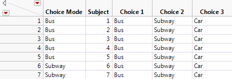
Make the Response Data Table
For the Response Data Table, you need the Subject and Choice Mode columns, but you also need a column for each possible choice.
3. With the original data table open, select the Subject and Choice Mode columns.
4. Select Tables > Subset.
5. Select Selected Columns and click OK.
Note the default table name is Subset of Daganzo Trip.
6. Select Cols > Add Multiple Columns.
7. For the Column prefix, type Choice. Type 3 next to How many columns to add. Click Numeric and select Character.
8. Click OK.
The columns Choice 1, Choice 2, and Choice 3 have been added.
9. Type “Bus” (without quotation marks) in the first row of Choice 1. Right-click the cell and select Fill > Fill to end of table.
10. Type “Subway” (without quotation marks) in the first row of Choice 2. Right-click the cell and select Fill > Fill to end of table.
11. Type “Car” (without quotation marks) in the first row of Choice 3. Right-click the cell and select Fill > Fill to end of table.
The resulting table is shown in Figure 5.47.
Figure 5.47 Partial Subset Table of Daganzo Data with Choice Set
Fit the Model
Now that you have separated the original Daganzo Trip.jmp table into two separate tables, you can run the Choice Platform.
1. Select Analyze > Consumer Research > Choice.
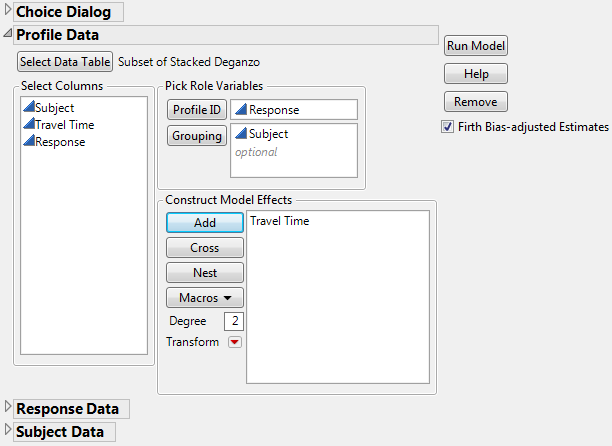
2. Specify the model, as shown in Figure 5.48.
Figure 5.48 Choice Dialog Box for Subset of Daganzo Data
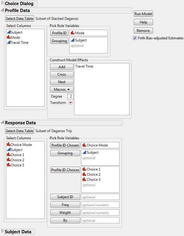
3. Click Run Model.
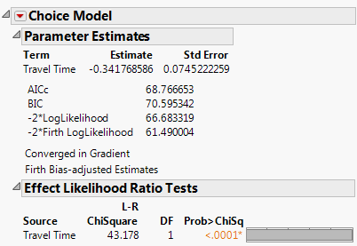
The resulting parameter estimate now expresses the utility coefficient for Travel Time and is shown in Figure 5.49.
Figure 5.49 Parameter Estimate for Travel Time of Daganzo Data
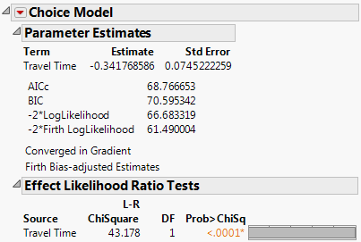
The negative coefficient implies that increased travel time has a negative effect on consumer utility or satisfaction. The likelihood ratio test result indicates that the Choice model with the effect of Travel Time is significant.
Example of Transforming Data to One Analysis Table
Rather than creating two or three tables, it can be more practical to transform the data so that only one table is used. For the one-table format, the subject effect is added as in the previous example. A response indicator column is added instead of using three different columns for the choice sets (Choice 1, Choice 2, Choice 3). The transformation for the one-table scenario includes the following steps.
1. Create or open Stacked Daganzo.jmp from the “Stack the Data” steps shown in “Example of Transforming Data to Two Analysis Tables”.
2. Select Cols > New Column.
3. Type Response as the Column Name.
4. Click Column Properties and select Formula.
5. Select Conditional under the Functions (grouped) command and select If from the formula editor.
6. Select the column Choice Mode for the expression (expr).
7. Enter “=” and select Mode.
8. Type 1 for the Then Clause and 0 for the Else Clause.
9. Click OK in the Formula Editor window. Click OK in the New Column window.
The completed formula should look like Figure 5.50.
Figure 5.50 Formula for Response Indicator for Stacked Daganzo Data
10. Select the Subject, Travel Time, and Response columns and then select Tables > Subset.
11. Select Selected Columns and click OK.
A partial listing of the new data table is shown in Figure 5.51.
Figure 5.51 Partial Table of Stacked Daganzo Data Subset
12. Select Analyze > Consumer Research > Choice to open the launch window and specify the model as shown in Figure 5.52.
Figure 5.52 Choice Dialog Box for Subset of Stacked Daganzo Data for One-Table Analysis
13. Click Run Model.
A pop-up dialog window asks whether this is a one-table analysis with all the data in the Profile Table.
14. Select Yes to obtain the parameter estimate expressing the utility Travel Time coefficient, shown in Figure 5.53.
Figure 5.53 Parameter Estimate for Travel Time of Daganzo Data from One-Table Analysis
Notice that the result is identical to that obtained for the two-table model, shown earlier in Figure 5.49.
This chapter illustrates the use of the Choice Modeling platform with simple examples. This platform can also be used for more complex models, such as those involving more complicated transformations and interaction terms.
Additional Examples of Logistic Regression Using the Choice Platform
Example of Logistic Regression Using the Choice Platform
Use the Choice Platform
1. Select Help > Sample Data Library and open Lung Cancer Responses.jmp.
Notice this data table has only one column (Lung Cancer) with two rows (Cancer and NoCancer).
2. Select Analyze > Consumer Research > Choice > Select Data Table > Lung Cancer Responses.jmp > OK.
3. Select Lung Cancer as the Profile ID and Add Lung Cancer as the model effect. The Profile Data window is shown in Figure 5.54.
Figure 5.54 Profile Data for Lung Cancer Example
4. Click the disclosure icon for Response Data > Select Data Table > Other > OK.
5. Open the sample data set Lung Cancer Choice.jmp.
6. Select Lung Cancer for Profile ID Chosen, Choice1 and Choice2 for Profile ID Choices, and Count for Freq. The Response Data launch window is shown in Figure 5.55.
Figure 5.55 Response Data for Lung Cancer Example
7. Click the disclosure icon for Subject Data > Select Data Table > Lung Cancer Choice.jmp > OK.
8. Add Smoker as the model effect. The Subject Data launch window is shown in Figure 5.56.
Figure 5.56 Subject Data for Lung Cancer Example
9. Uncheck Firth Bias-adjusted Estimates and Run Model.
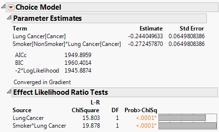
Choice Modeling results are shown in Figure 5.57.
Figure 5.57 Choice Modeling Logistic Regression Results for the Cancer Data
Use the Fit Model Platform
1. Select Help > Sample Data Library and open Lung Cancer.jmp.
2. Select Analyze > Fit Model.
Automatic specification of the columns is: Lung Cancer for Y, Count for Freq, and Smoker for Add under Construct Model Effects. The Nominal Logistic personality is automatically selected.
3. Click Run.
The nominal logistic fit for the data is shown in Figure 5.58.
Figure 5.58 Fit Model Nominal Logistic Regression Results for the Cancer Data
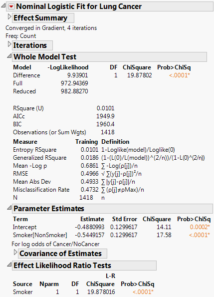
Notice that the likelihood ratio chi-square test for Smoker*Lung Cancer in the Choice model matches the likelihood ratio chi-square test for Smoker in the Logistic model. The reports shown in Figure 5.57 and Figure 5.58 support the conclusion that smoking has a strong effect on developing lung cancer. See the Logistic Regression chapter in the Fitting Linear Models book for more details.
Example of Logistic Regression for Matched Case-Control Studies
This section provides an example using the Choice platform to perform logistic regression on the results of a study of endometrial cancer with 63 matched pairs. The data are from the Los Angeles Study of the Endometrial Cancer Data in Breslow and Day (1980) and the SAS/STAT(R) 9.2 User's Guide, Second Edition (2006). The goal of the case-control analysis was to determine the relative risk for gallbladder disease, controlling for the effect of hypertension. The Outcome of 1 indicates the presence of endometrial cancer, and 0 indicates the control. Gallbladder and Hypertension data indicators are also 0 or 1.
1. Select Help > Sample Data Library and open Endometrial Cancer.jmp.
2. Select Analyze > Consumer Research > Choice.
3. Click the Select Data Table button.
4. Select Endometrial Cancer as the profile data table. Click OK.
5. Assign Outcome to the Profile ID role.
6. Assign Pair to the Grouping role.
7. Add the following columns as model effects: Gallbladder, Hypertension.
8. Deselect the Firth Bias-Adjusted Estimates check box.
9. Select Run Model.
A pop-up dialog window asks whether this is a one-table analysis with all the data in the Profile Table.
10. Click Yes.
11. On the Choice Model red triangle menu, select Utility Profiler.
The report is shown in Figure 5.59.
Figure 5.59 Logistic Regression on Endometrial Cancer Data
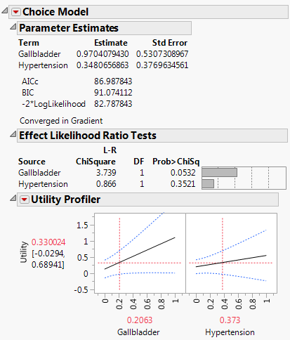
Likelihood Ratio tests are given for each factor. Note that Gallbladder is nearly significant at the 0.05 level (p-value = 0.0532). Use the Utility Profiler to visualize the impact of the factors on the response.
Statistical Details
Parameter estimates from the choice model identify consumer utility, or marginal utilities in the case of a linear utility function. Utility is the level of satisfaction consumers receive from products with specific attributes and is determined from the parameter estimates in the model.
The choice statistical model is expressed as follows:
Let X[k] represent a subject attribute design row, with intercept
Let Z[j] represent a choice attribute design row, without intercept
Then, the probability of a given choice for the k'th subject to the j'th choice of m choices is:
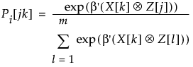
where:
‒ ⊗ is the Kronecker rowwise product
‒ the numerator calculates for the j'th alternative actually chosen
‒ the denominator sums over the m choices presented to the subject for that trial
..................Content has been hidden....................
You can't read the all page of ebook, please click here login for view all page.