Chapter 11: Causality Tests for the Danish Egg Market

Introduction

The Danish Egg Market

Formulation of the VARMA Model for the Egg Market Data

Estimation Results

Model Fit

Causality Tests of the Total Market Series

Granger Causality Tests in the VARMAX Procedure

Causality Tests of the Production Series

Causality Tests That Use Extended Information Sets

Estimation of a Final Causality Model

Fit of the Final Model

Conclusion

Introduction

In this chapter, some historical time series for the Danish egg market are analyzed. The analysis is intended to study the interdependence between the price of eggs and the production of eggs. Economic theory says that increasing prices lead to increasing production, and increasing production leads to decreasing prices. The example is chosen to demonstrate how the VARMAX procedure is used for testing causality.

You will see that the production series seems to affect the price series and that this effect includes lags but not vice versa. When you see a lagged effect one way but not the other way, the situation is intuitively a causality because the reason comes before the reaction. This situation is a simple example of Granger causality. The hypothesis is easily tested by using PROC VARMAX.

Two series for general Danish agricultural production are included in the analysis, leading to a total of four time series. In this setup, the Granger Causality is extended to allow for different information sets.

The Danish Egg Market

In this section, a Vector Autoregressive Moving Average (VARMA) model is estimated for four monthly series that are related to the Danish egg market in the years 1965–1976.

You will find the data series in the data set EGG in the library SASMTS. The data set consists of four series of 144 observations:

•   QEGG is an index of the produced quantity of eggs.

•   PEGG is an index of the price of eggs.

•   QTOT is an index of the quantity of the total agricultural production.

•   PTOT is an index of the price of the total agricultural production.

•   DATE is the month of the observation in a SAS date variable. The date is programmed as the 15th of every month, but the format prints only the month.

All series are published as indices, so they are all measured in the same unit. In other words, units are of no importance.

Program 11.1 plots the four series in an overlaid plot using PROC SGPLOT. The four series are plotted with different markers and colors.

Program 11.1: Plotting the Four Series Using PROC SGPLOT.

You can see in Figure 11.1 that the series, at least to some extent, have trends and that seasonal effects are present, which is to be expected. Classical Box-Jenkins techniques identify that a first-order difference should be applied to explain the trends, and seasonal AR models can be used for the seasonality. In the following sections, the series are analyzed using the facilities in PROC VARMAX.

Figure 11.1: An Overlaid Plot of the Four Series

Formulation of the VARMA Model for the Egg Market Data

In the plot of the price series (Figure 11.1), it is obvious that the price rose rapidly in the first months of 1973. This is a well-established fact because Denmark entered the European Union on January 1, 1973, mainly in order to help the farmers. Events with such a significant and easily understood impact on the time series are best modeled as exogenous. In this situation, the effect is seen in positive changes of the price index series for some months. One way to model this is simply to include dummy variables for the event, by the variable EUDUMMY in Program 11.2. This variable is then applied only for the total price series. The four variables are separated by commas in the MODEL statement to make sure that the right side variable EUDUMMY applies only to the left side variable PTOT.

In this example, the same order of differencing is applied to all four series. This is mainly because it is easier to understand the final model if all the series in the model are of the same integration order. The order of differencing is explicitly stated for each of the four series in the parentheses after the DIF option.

Of course, monthly data for time series from the agricultural sector includes seasonality patterns. An easy way to correct for the seasonality in the model is to include seasonal dummies. This method gives a model for deterministic seasonality. This is in contrast to stochastic seasonal effects, which are modeled by multiplicative seasonal models. In the application of PROC VARMAX in Program 11.2, seasonal dummy variables are included with the option NSEASON=12 to the MODEL statement (in this example, for monthly observations). The option NSEASON=12 establishes 11 dummy variables using the first available month in the estimation data set as the reference. This method of using dummies is usually applied to model seasonality by PROC VARMAX. Multiplicative Seasonal models are not supported by PROC VARMAX because they are too involved in the case of multivariate series.

The option LAGMAX=25 in the MODEL statement states that residual autocorrelations and portmanteau tests of model fit are calculated for lags up to 25 and not just up to the default value, LAGMAX=12. This higher value is chosen because model deficits for seasonal time series are often seen around lags twice the seasonal length, which is 12 in this particular model.

The choice of the order, p, for the autoregressive part and the order, q, for the moving average part of the VARMA(p,q) model can be determined in many ways. The automatic detection of model order is technically hard to perform in this situation because estimating a model that includes both autoregressive and moving average terms, p > 0 and q > 0, produces numerically unstable results. The number of parameters is huge, having 12 seasonal dummies for each of the four series and 16 extra parameters for each lag in the autoregressive model. So the order of the autoregressive is chosen as p = 2. In the DATA step in Program 11.2, the dummy variable EUDUMMY is defined. In Program 11.2, this intervention is allowed to act with up to 3 lags by the option XLAG=3 because the effect was not immediate but rather spread over some months. The application of PROC VARMAX in Program 11.2 includes all these mentioned options.

Program 11.2: Defining a Dummy Variable and a Preliminary Estimation of a VARMA(2,0) Model

Estimation Results

The model contains many parameters, but the schematic presentation (Output 11.1) gives the overall picture. In Output 11.1, the periods (.) indicate insignificant parameters; the signs + and - indicate significant parameters at a 5% level. Many parameters are insignificant, which leads to the conclusion that the autoregressive part of the model is over-parameterized. The many stars (*) for the exogenous variable EUDUMMY denote parameters that are excluded from the model because the variable EUDUMMY in Program 11.2 affects only the last variable—that is, the total price variable PTOT. In the output, XL0, XL1, and so on are short for eXogenous at lags 0, 1, and so on.

Output 11.1: Schematic Presentation of the Significant Parameters

Model Fit

This second-order autoregressive model, however, gives a satisfactory fit to the first 25 residual autocorrelations and cross-correlations, as displayed schematically in Output 11.2. (Output 11.2 presents the correlations only up to lag 12.) Few elements are significantly different from zero because they are numerically larger than twice their standard error. This is indicated by – or + in the schematic representation of the residual autocorrelations in Output 11.2. The remaining cross-correlations are all insignificant at a 5% level, which is indicated by a period (.) in Output 11.2. The major problem is found at lag 11. Portmanteau tests for cross-correlations in the residuals reject the model fit because the squares of the many minor cross-correlations are accumulated. The output of the portmanteau tests for lags up to 25 are too voluminous to quote in this text.

Output 11.2: Significance of the Cross-Correlations

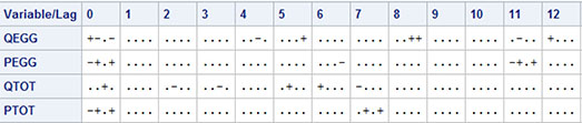
Of course, the fit gets better if the model is extended by autoregressive parameters for lag 11 and 12, but this would be a severe over-parameterization. The lack of fit can also be mended if some minor outliers are taken into account in the model. But all such remedies for repairing a lack of fit that do not point at specific, important model failures seem to be a waste of energy.

The model includes many parameters that have to be estimated: 2 ×16 autoregressive parameters and 4 ×11 seasonal dummy parameters, 4 parameters for the EUDUMMY, and a residual covariance matrix. So the table of estimates is not shown here because it is evident that the model is heavily over-parameterized, when every series affects all series at lags 1 to 2 in the autoregressive part. Moreover, the seasonal structure is not that significant. Far too many nonsignificant parameters are included in the model.

As in Chapter 9, it is then natural to test whether many parameters are superfluous to the model fit. When judged from Output 11.1, such testing could lead to a four-dimensional autoregressive model of order p = 2 for the QTOT variable. But for the other three series, the model order is probably much lower. The technique behind this form of model selection is demonstrated for the two-dimensional model in Chapter 9, so this will not be pursued in this chapter. Instead, we will rethink the purpose of the model building and in this way formulate some model simplifications in the next section.

Causality Tests of the Total Market Series

The Danish production of eggs is very small compared with the other sectors of Danish agricultural production. This means that it is impossible that the size and pricing at the egg market could have any influence on the size and pricing of the total agricultural production. On the other hand, it is natural to think that the egg market is influenced by the overall state of the total agricultural market.

In econometric terms, the total agricultural production is probably exogenous to the egg market. Intuitively, the term exogenous means that a variable is generated outside the model at hand. A typical example is that the oil price in the world market can affect the price of bus tickets in Copenhagen; but the price of bus tickets in Copenhagen can in no way affect the oil price. But in econometric theory, the discussion of exogeneity is more involved than this simple example.

In the present context, this possible causality means that it is pointless to set up a simultaneous model for all four series. Two models, one for the two-dimensional total agricultural market and one for the two-dimensional egg market, suffice. If only the egg market is of interest, the model for the total agricultural market is of no direct interest. Then the output of the total agricultural market can be taken as input to the model for the egg market. In regression terms, the two series for the total agricultural market can be included as right side variables in the model for the egg market. A model of this kind with the total agricultural market as a right side variable is an example of the X in the name of PROC VARMAX because the right side variable is considered as eXogenous.

However, testing is necessary to determine whether this is the case. According to the model structure, the immediate impact from the total agricultural market of the egg market is modeled by the four-dimensional covariance matrix for the four remainder terms. Such correlations are by nature not directly interpreted as causal, because correlation can be directed both ways. If some of the coefficients that correspond to effects from the egg market series to the total agricultural market series are different from zero, the present status of the egg market has influence on future values of the total market. If this is the case, the total market for agricultural products cannot be exogenous.

The hypothesis of a lagged effect is tested by testing the hypothesis that a particular two-by-two block of every autoregressive coefficient matrix is zero. In a formal mathematical formulation, causality from the series X₃ and X₄ (the series for the total Danish agricultural production) for the variables X₁ and X₂ (the series for the Danish egg market) is expressed as follows. The basic model is a VARMA(p,0) model:

$$X_t-{\phi }_1{X}_{t-1}-\mathrm{..}-{\phi }_p{X}_{t-p}={\epsilon }_t$$

The coefficients φ_m are given as follows:

${\phi }_m=\left(\begin{array}{cccc}{\text{φ}}_{m11}& {\text{φ}}_{m12}& {\text{φ}}_{m13}& {\text{φ}}_{m14}\\ {\text{φ}}_{m21}& {\text{φ}}_{m22}& {\text{φ}}_{m23}& {\text{φ}}_{m24}\\ 0& 0& {\text{φ}}_{m33}& {\text{φ}}_{m34}\\ 0& 0& {\text{φ}}_{m43}& {\text{φ}}_{m44}\end{array}\right)$

The 2 ×2 block of zeros in the lower left corner of the autoregressive matrix, φ_m, represents the parameters for lagged effects of the egg series, X₁ and X₂, to the total production series X₃ and X₄. The hypothesis is that all such parameters are insignificant.

This hypothesis is the same as testing the so-called Granger causality. The idea of the original Granger papers (1969 and 1980) is that causality is present if one group of series affects another group with a time delay, but not the other way around. In more informal terms, the term “Granger cause” is used. The causality, however, depends on what is known—that is, which series the model includes besides the series of the causal relation.

Granger Causality Tests in the VARMAX Procedure

The test statistic for Granger causality is calculated by Program 11.3. The CAUSAL statement explicitly specifies that the group 1 variables cause the group 2 variables. More precisely, the hypothesis is that all coefficients that represent lagged effects of the group 2 variables to the group 1 variables equal zero. As demonstrated by Program 11.4, this is the same as testing whether a specific corner of all autoregressive matrices is zero.

Program 11.3: Granger Causality Testing by PROC VARMAX

In the output element “Granger Causality Wald Test” in Output 11.3, it is seen that the hypothesis is accepted p = .29.

Output 11.3: Results of the Granger Causality Test

This test for Granger causality is equivalent to testing the hypothesis that the lower, left 2 ×2 corners of the autoregressive coefficient matrices in Output 11.1 are zero. The hypothesis of Granger causality can alternatively be tested by an explicit specification of the zero elements in the matrices as in Program 11.4.

Program 11.4: Testing Hypothesis of Causality Directly

In Output 11.4, it is seen that the testing results are equal to the test results of the Granger causality in Output 11.3, although the reported test statistic s is not exactly equal. The notion of Granger causality and the causal statement in PROC VARMAX are, in this light, only a smart way to drastically reduce the number of parameters. But by intuition, this test setup serves two purposes: it reduces the number of parameters, but it it also tells the user something important about the data series.

Output 11.4: Simultaneous Test Results for Program 11.4

The conclusion of this part of the analysis is that the two series relating to the total agricultural production in Denmark, QTOT and PTOT, do Granger-cause the series for the egg production QEGG and PEGG. For this reason, QTOT and PTOT can be specified as independent variables in models for the egg market, because their own statistical variation is of no interest for the models of the eggs. If the series QTOT and PTOT for total production are included as right side variables in a model for the two egg series QEGG and PEGG, then they are considered deterministic in the model, and the model then has nothing to tell about their statistical variation. You could say that these two series for the total agricultural production are exogenous. For proper definitions of various forms of the concept of exogeneity, see Engle, Hendry, and Richard (1983).

Causality Tests of the Production Series

In the following application of PROC VARMAX (Program 11.5), the series QTOT and PTOT are used as right side variables in the model statement. Because the exogenous variables apply to both output series, no separation of the right side variables by commas is needed. The number of lags of the input series is specified as 2 by the option XLAG=2 in the model statement. This lag length applies to both input series. In this model, the variable PTOT is used as an independent variable. This is the reason that the dummy variable for EU membership is unnecessary in this application.

Program 11.5: Specifying Exogenous Variables

Output 11.5 presents the estimated autoregressive parameters as matrices in a table. The estimated autoregressive parameters tell us that the series PEGG is influenced by the series QEGG at lag one and two because φ₁₂₁ = AR(1,2,1) = −1.50 and φ₂₂₁ = AR(2,2,1) = − .61 are both negative. The negative sign tells that if the production increases, then in most cases the price will decrease. In this case, the lower price also is seen to include lagged effects up to lag 2 . But this presentation in matrix form shows that no important lagged influence is present for the price series PEGG to the production series QEGG.

Output 11.5: The Autoregressive Parameters Shown in Matrix Form

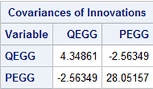
This argument says nothing about the correlation at lag zero, which is estimated to ρ =  −.23. But this correlation can be directed both ways because no lags are involved. This correlation matrix for the residual series is printed as the lag zero part of the cross-correlation function. The correlation, −.23, is easily calculated from the printed covariance matrix for the innovations (Output 11.6), as follows:

$$\text{ρ=}\frac{-2.56}{\sqrt{4.35\times 28.05}}=-.23$$

Output 11.6: The Error Covariance Matrix

Causality Tests That Use Extended Information Sets

The findings from Output 11.5 can once again be interpreted as a Granger causality, this time showing that the produced quantity of egg Granger-causes the price of egg. This conclusion is drawn because no lagged effect of the price series is included in the model for the produced quantities of the series. In the model, the total market for agricultural products is included as right side variables. So the conclusion is drawn when the egg series are adjusted by observations of the total market for agricultural products. In the notation of Granger causality, it is then said that the causality of the produced quantity of eggs to the price of eggs is present in the information set defined by the two series for the total market for agricultural products.

This hypothesis is tested by Program 11.6, again using a causality statement. For comparison, the opposite hypothesis that the production does not Granger-cause the price is also tested by the second application of PROC VARMAX in Program 11.6.

Program 11.6: Testing the Direction of Causalities Between the Price and the Quantity Series

The Outputs 11.7 and 11.8 show that the p-value for the first test is as high as p = .64, while the hypothesis in the second test is rejected with a p-value below .0001. You can then conclude that the production series, QEGG, does in fact Granger-cause the price series, PEGG, but not vice versa. This conclusion is drawn while controlling for the effect of production and price series for the total agricultural market because they are used as right side variables in the model estimated by Program 11.6 for both egg series.

Output 11.7: Testing Causality of the Quantity Series

Output 11.8: Testing Causality of the Price Series

This direction of the causality is understandable because prices can be quickly adjusted, but the production is difficult to change. This means that high production quickly leads to lower prices; but the production facilities have difficulties in increasing the production when the prices are increasing.

Estimation of a Final Causality Model

The model that also uses the produced quantity of eggs, QEGG, as a right side variable is estimated in Program 11.7. It turns out that some of the parameters in this model can be set to zero. For instance, the explanatory variable QTOT for the total Danish agricultural production is unnecessary in the model because it affects none of the egg series. In Program 11.7, a test for this hypothesis is further included in the TEST statement.

In the TEST statement, the (1,2) entries of the matrix of parameters for the exogenous variables at lags 0, 1, and 2 are all hypothesized to 0. The (1,2) entries are the parameters  from the second exogenous parameter to the first (the only) endogenous variable. The notation for the exogenous variables is that, for instance, XL(2,1,2) is the coefficient at lag 2 to the first endogenous (the right side variable) from the second exogenous variable (left side variable).

Program 11.7: Testing the Significance of the Total Production Series

The hypothesis that the total Danish agricultural production has no impact whatsoever on the Danish market for eggs is clearly accepted. (See Output 11.9.) This means that the series is irrelevant if the effect of the interrelations between the price and production of eggs on the total market is under study. Only the prices at the total agricultural market have some impact on the egg market.

Output 11.9: Test Results for the Exclusion of the Series QTOT from the Egg Market Model

The final model is estimated in Program 11.8 where only a single dependent variable is found on the left side because all other variables are proved to be exogenous right side variables.

Program 11.8: The Final Application of PROC VARMAX for the Egg Market Example

The estimated parameters of the resulting model are given in Output 11.10.

Output 11.10: The Estimated Parameters from the Final Model

Fit of the Final Model

The model fit is accepted according to the autocorrelations (ACF), the inverse autocorrelations (IACF), and the partial autocorrelations (PACF) of the residuals of the model for the differenced price of eggs series. (See Figure 11.2.) These plots are a part of the output produced by Program 11.8.

Figure 11.2: Residual Autocorrelations in the Model of the Differenced Price Series

This series is the only series that is modeled in this application of PROC VARMAX because the other series are all accepted by statistical tests to be deterministic right side variables in the model for this series. The fit of the model is further accepted by the tests for normality and Autoregressive Conditional Heteroscedasticity (ARCH) effects. (See Output 11.11.)

Output 11.11: Tests for Normality and ARCH Effects

Conclusion

In this chapter, a vector time series of dimension 4 is reduced to a model for just a single time series using the other 3 variables as exogenous, right side variables. This is possible because no lagged effects from the single left side variable to the other variables exists in the final model. In other words, no feedback exists in the system. The only possible effects from the left side variables to the right side variables are hidden in the lag 0 covariance matrix because correlations have no directions.

The reduction of the model is easy to understand with use of the concept of Granger causality. This reduction is similar to a simultaneous testing of the significance of many parameters in an involved 4-dimensional VARMA model. Such testing of causality is possible with use of PROC VARMAX.