Chapter 13: Vector Error Correction Models

Introduction

The Error Correction Model

The Matrix Formulation of the Error Correction Model

The Long-Run Relation

A Simple Example: The Price of Potatoes in Ohio and Pennsylvania

A Simple Regression

Estimation of an Error Correction Model by PROC VARMAX

Dickey-Fuller Test Results

Estimated Error Correction Parameters

The αβ^T Matrix

Properties of the Estimated Model

The Autoregressive Terms in the Model

Theory for Testing Hypotheses on β Parameters

Tests of Hypotheses on the β Parameters Using PROC VARMAX

Tests for Two Restrictions on the β Parameters

Estimated α Parameters under the Restrictions

Tests of Hypotheses on the α Parameters by PROC VARMAX

The TEST Statement for Hypotheses on the α Parameters

The RESTRICT Statement for the β Parameters

Restrictions on Both α Parameters and β Parameters

Properties of the Final Model

Conclusion

Introduction

In this chapter, the vector error correction model is introduced and demonstrated with examples. First, the underlying theory is outlined in brief without many mathematical details. The underlying idea in error-correction modeling is that some stability restriction is assumed to exist, and the VARMAX procedure is then applied to estimate a model that allows for such a situation.

The theory, when thoroughly evolved, depends heavily on matrices, but this notation is avoided as much as possible. Instead, the models are described in the form of separate equations that give the idea in simple examples. However, it has to be stressed that PROC VARMAX can handle the general situation, and some of the syntax also depends on the matrix notation. So this notation cannot be 100% neglected.

Chapter 14 takes the subject further by introducing the concept of cointegration, testing for the existence of error corrections, rank restrictions, and so on. In this chapter, these relations are assumed to exist by pure intuition. Also, in Chapter 14, the theory is kept at a minimum, and the subject is mainly demonstrated by examples using PROC VARMAX. In short, cointegration theory can be applied to establish the existence of relations that can be used for error-correction models.

The theory is, of course, important, and the reader is referred to the rich literature, See, for instance, Juselieus (2006) or Johansen (1995) for textbook references.

The Error Correction Model

As a simple example, consider two time series x_t and y_t. Assume that some simple linear relation is often seen between these two series:

y_t + β₂x_t + β₀ ~ 0

The sub-indices on the β parameters are chosen because of the matrix notation. The matrix notation is necessary for testing hypotheses such as, for example, the hypothesis β₀ = 0. The order of the terms is in accordance with the matrix notation. Note that the sign of β₂ is the opposite to the sign of the coefficient to x_t in a regression of y_t on x_t.

Examples might be the price of crude oil in Europe and in the United States. Of course, the prices are not exactly equal by definition, but it is plausible that an approximately linear relation could be established by global trading mechanisms. Many theories in, for example, economics or physics assume that such relations exist, but without saying that equality is observed at every point in time. The relation is for that reason often denoted a long-run equality or in economic terms an equilibrium.

Later, a coefficient β₁ to y_t is introduced, and the equations in this section are found by dividing by β₁ in this more general relation:

β₁y_t + β₂x_t + β₀ ~ 0

This relation is supposed to be a well-established fact even if the values of the β parameters are not exactly known. Chapter 14 demonstrates how to identify and test for the existence of such relations.

If the long-run relation for some reason is disturbed such that

y_t + β₂x_t + β₀ ≠ 0

then the economic market or the laws of physics will tend to seek toward the relation by changing the values of x_t and y_t in the direction of the equation again. This tendency to move toward the relation can be modeled by letting the degree of instability at time t − 1 be an independent variable for the next observations of x_t and y_t:

z_t−1 = y_t−1 + β₂x_t−1 + β₀

This could be modeled as follows:

y_t =  y_t−1 + α₁( y_t−1 + β₂x_t−1 + β₀ ) + ...

and

x_t =  x_t−1 + α₂( y_t−1 + β₂x_t−1 + β₀ ) + ...

where more terms can be included in the model as indicated by the dots at the ends of the equations.

The rationale behind this expression is that if the relation is not met at time t − 1, then the series x_t and y_t will react by trying to reestablish the relation at time t.

To see this, assume that α₂ is positive and then if

z_t−1 = y_t−1 + β₂x_t−1 + β₀ > 0

the x series will increase from time t − 1 to t by α₁z_t−1. Similarly, if α₁ is negative, the y series will decrease by α₂z_t−1. Both reactions are in the direction of the long-run relation to hold.

The α parameters show how fast the reestablishment of the stable relation happens. This can be very fast, almost immediately at a stock market exchange, or take many decades in the economic integration of the countries in the European Union.

The Matrix Formulation of the Error Correction Model

This model can be written in matrix form like a usual VARMAX model. In order to do so, denote the first order differences Δx_t = x_t − x_t−1 and Δy_t = y_t − y_t−1 leading to the bivariate differenced process:

$$\Delta y_t=\left(\begin{array}{c}\Delta y_t\\ \Delta x_t\end{array}\right)$$

And define the matrices α of dimension 2 ×1and β of dimension 3 ×1 as

$$\text{α}=\left(\begin{array}{c}{\alpha }_1\\ {\alpha }_2\end{array}\right),\text{β}=\left(\begin{array}{c}{\beta }_1\\ {\beta }_2\\ {\beta }_0\end{array}\right)$$

which makes the matrix αβ^T a 2 ×3 matrix. Note that the last entry in β is the constant term β₀ in the long-run relation. In the model this is the coefficient to the number 1 in the terms for the lagged value for time t − 1.

The model is then written as a VARMAX model for Δy_t:

$$\Delta y_t=\left(\begin{array}{c}\Delta y_t\\ \Delta x_t\end{array}\right)={\text{αβ}}^T\left(\begin{array}{c}{y}_{t-1}\\ x_{t-1}\\ 1\end{array}\right)+\mathrm{...}$$

The entries of the matrix product αβ^T are coefficients to an independent variable in a usual VARMAX model—the X part of VARMAX for exogenous. This model can be extended as indicated by the periods “...”. A VARMA model can be stated with autoregressive or moving average terms. Also, seasonal dummy variables and other exogenous variables can be included. The point is that the entries in the basic coefficient matrices α and β are not the direct parameters in the model. Instead, the matrices are sums and products of the α’s and β’s in the expression. This is not a typical time series model because the parameterization is nonlinear.

But it is possible to estimate the α and β parameters anyway if some assumptions are met. In short, the series should have unit roots. That is, they should need a first-order differencing in order to be stationary. See Chapter 5. The assumptions of unit roots are tested by, for example, Dickey-Fuller tests as shown in Chapter 5.

The Long-Run Relation

The residuals z_t in the long-run relation shown below should form a stationary time series.

z_t = y_t + β₂x_t + β₀

This is just the meaning of saying that the relation is stable. The hypothesis of stationarity of the residuals forms a more complicated test situation because the β parameters must be estimated. Such tests are described in Chapter 14.

This simple presentation can be generalized to more than two series and more than one linear stable relation. Also, trends can be included in various ways. One special point is that the model structure depends on whether an intercept is included in the long-run relation like it is in the formulas above. This intercept term can be excluded or perhaps replaced by a linear trend.

The question how to determine the number of such relations and to specify their precise form is the subject of cointegration testing, which is the subject of Chapter 14. In this chapter it is mainly assumed that one or more of relations of this form exist using arguments based on intuition.

A Simple Example: The Price of Potatoes in Ohio and Pennsylvania

The data set POTATOES_YEAR includes prices for potatoes in several states in the United States back to 1866 and up to 2013. The variables are named by the name of the state. The prices are the logarithmically transformed price. The original price is the total value of the production of potatoes within the state divided by the produced quantity. The unit of the price is US Dollar per CWT (approximately 45 kg), but the precise unit of measurement is of no importance because of the transformation by logarithms.

In this section, only the series for prices in Ohio and Pennsylvania are used. The two series are plotted by two applications of PROC SGPLOT in Program 13.1. Program 13.1 also includes the code for fitting a simple regression between the two series.

Program 13.1: Simple Plots and Analyses Price for Potatoes in Ohio and Pennsylvania

It is evident from the plot that the two series are almost equal. Minor discrepancies exist, but it is not like one price is systematically larger than the other. A quick graphical judgment clearly tells you that an approximately linear relation exists. Also, an assumption of a stable price relation between these two time series of prices is intuitively correct in an economic context.

Figure 13.1: Plot of the Log-Price of Potatoes in Ohio and Pennsylvania

A Simple Regression

The second plot generated by PROC SGPLOT in Program 13.1 is a regression plot using the price in Pennsylvania as independent variable and the price in Ohio as the dependent variable. At the plot, the points are labeled by the year with the option DATALABEL=YEAR. It is obvious that the (log-transformed) price is much larger for the last years of the observation period than for the first years. A simple regression like the one in Program 13.1 does not then, of course, lead to a valid model that tells all in this situation. But the plot, Figure 13.2, clearly shows that a linear relation should in some way be included in a model for the two series.

Figure 13.2: Plot of the Two Series as a Regression

The estimated regression line in Figure 13.2 has the equation

y_t + β₂x_t + β₀ = 0

where y_t denotes the price in Ohio, and x_t is the price in Pennsylvania. The parameters from the application of PROC REG in Program 13.1 are β₁ = −.977 and β₂ = −.006 after the signs are changed according to the present notation for regression. See Output 13.1. Note, however, that autocorrelation problems exist in this regression, which is estimated by ordinary least squares as the Durbin-Watson test gives significance. This means that the reported standard deviations are misleading. But remembering this, it is clear that the estimated regression is indeed very close to the identity line y_t = x_t because the coefficient to x_t, −.977, is very close to 1.

Output 13.1: Estimated Regression Parameters

Estimation of an Error Correction Model by PROC VARMAX

Program 13.2 gives a first application of PROC VARMAX to a model for these two price series, using a regression with an intercept as the long-run relation. The long-run relation is stated in a COINTEG statement that can be used to specify much more advanced models, as will be demonstrated later. In this application, it suffices to state that only one linear stable relation exists and that the variable OHIO is considered as the left side variable with a regression coefficient equal to 1 (that is, no coefficient) when the linear long-run relation is reported. The intercept in the long-run relation is included by the option ECTREND to the COINTEG statement.

Note that in SAS/ETS 14.1 and earlier versions, the intercept in the long-run relation was included by the option ECTREND to the ECM option to the MODEL statement, where also the number of relations, here just 1, was mandatory. The MODEL statement, before SAS/ETS14.1, had to be in the following form:

MODEL OHIO PENNSYLVANIA/P=4 Q=0 ECM=(RANK=1 NORMALIZE=OHIO ECTREND);

Program 13.2: Fitting an Error Correction Model with an Intercept

Dickey-Fuller Test Results

In error correction models, it is implicitly assumed that the series have unit roots and that they must be differenced in order to meet stationarity. The Dickey-Fuller tests for this hypothesis are presented in Output 13.2. The hypothesis of unit roots is accepted for the situation with a constant mean. But a model with an imposed linear trend and stationary residuals is also a possibility.

Output 13.2: Results of Dickey-Fuller tests for Stationarity

Estimated Error Correction Parameters

The estimated α parameters and β parameters are given in Output 13.3. The β parameters are numerically close to, but not exactly equal to, the regression parameters listed in Output 13.1. Note that the β parameters are identified by the name of the independent variable. Accordingly, the intercept is identified by the variable name (just the number 1), which is the independent variable that corresponds to an intercept. The reported relation is normalized such that the coefficient to the y_t variable, which is the price in Ohio, is set to 1. This is programmed by the option NORMALIZE=OHIO to the COINTEG statement in Program 13.2. This normalization makes the reported long-run relation look like the regression in Output 13.1.

Output 13.3: Estimated α Parameters and β Parameters

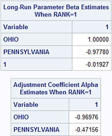
Output 13.4 gives another part of the output, which presents the estimated α and β parameters. The actual values of these parameters are determined by the normalization by letting β₁ = 1. Standard deviations are supplied only for the α parameters. Note that these standard deviations are based on asymptotics, so it is unlikely to be correct, by using only Output 13.4, that the parameter α₂ equals 0. But it is obvious from Output 13.4 that the adjustment factor is larger for the first series (the Ohio price series) than for the second series (the Pennsylvania price series).

Output 13.4: Estimated α and β Parameters

The αβ^T Matrix

These estimated α and β parameters lead to the αβ^T matrix, which is also printed in the procedure output. See Output 13.5. This matrix is the actual matrix in the model equation for Δy_t:

$$\Delta y_t=\left(\begin{array}{c}\Delta y_t\\ \Delta x_t\end{array}\right)=\alpha {\beta }^T\left(\begin{array}{c}{y}_{t-1}\\ x_{t-1}\\ 1\end{array}\right)+\mathrm{...}$$

Output 13.5: The αβ^T Matrix

Note that this αβ^T matrix is invariant under the normalization of the β parameters, letting β₁ = 1. The matrix is the same if the normalization is used for the Pennsylvania series instead. Even if no normalization is used, the αβ^T matrix remains the same.

The estimated α and β parameters change drastically if the option NORMALIZE=OHIO is omitted from Program 13.2. Output 13.6 gives the results.

Output 13.6: Estimated α Parameters and β Parameters without Normalization

The log likelihood of the fitted model is the output part entitled “Mutilvariate Diagnostics” in the printed results. The table is just one number. See Output 13.7.

Output 13.7: The Log-Likelihood of the Estimated Model

Properties of the Estimated Model

The error correction part of the model is given by the equations

y_t =  y_t−1 − .97( y_t−1 − .98x_t−1 − .02 ) + ...

for the Ohio price series and

x_t =  x_t−1 − .47( y_t−1 − .98x_t−1 − .02 ) + ...

for the Pennsylvania price series.

These relations are understood as follows. Assume that the long-run relation is wrong at time t – 1 such that

y_t−1 − .98x_t−1 − .02 > 0

Then the values of both price series x_t and y_t are reduced from time t − 1 to t because of the negative coefficients outside the parentheses. But in the y_t series, the Ohio price series is reduced the most. This is because the coefficient β₁ = .98 (note that it is written with a minus sign −.98 in Output 13.3) is numerically larger than the coefficient .47 for the Pennsylvania series x_t. In total, the values of x_t and y_t tend to reduce the imperfections of the long-run relation at time t compared to time t − 1.

In approximate terms, the coefficient .98 in the long-run relation is considered to equal 1, and the intercept in the long-run can be ignored. Then, the error in the long-run equation y_t − x_t is halved when compared to the error y_t−1 − x_t−1 at time t − 1. These two hypotheses upon the coefficients in the long-run equation are in fact accepted by testing in the next section.

The Autoregressive Terms in the Model

In Program 13.2, autoregressive parameters up to lag 4 are estimated by the option P=4. Most of these estimated autoregressive parameters are in fact insignificant as seen in Output 13.8. But a few of them are necessary in order to have a fit of the model without residual autocorrelation, which is otherwise present in the Pennsylvania price series. It is possible to gain some statistical efficiency by excluding superfluous parameters in this situation. But this will not be pursued in this context. See Chapter 9. Moreover, the model fit should also be tested. Again, see Chapter 9.

Output 13.8: Estimated Autoregressive Parameters

Theory for Testing Hypotheses on β Parameters

One conclusion of the simple example in the previous section was that the intercept in the long-run equation was very close to 0 and that the coefficient to the Pennsylvania price series was very close to 1. If both these hypotheses are accepted, then the long-run relation is that the price of potatoes in Ohio and in Pennsylvania is the same and that deviations from this equation are reduced fast. In this section, you will see how such hypotheses are estimated by PROC VARMAX.

It is possible to test linear hypotheses for both the α and β parameters in an Error Correction Model. A hypothesis has the form that the α and β parameters depend on fewer parameters in a way described in this section. Stating that the α and β parameters have a specific form is equivalent to saying that the α and β parameters meet some restrictions.

In the error correction model, the α and β parameters are formulated as vectors. In the model considered in the introduction in this chapter, they have the following form:

$$\alpha =\left(\begin{array}{c}{\alpha }_1\\ {\alpha }_2\end{array}\right),\beta =\left(\begin{array}{c}{\beta }_1\\ {\beta }_2\\ {\beta }_0\end{array}\right)$$

that is, 2 ×1 resp. 3 ×1 matrices. Here, the parameter β₁ is included even if the reported estimates in Output 13.3 are normalized to β₁ = 1.

The hypotheses then have the following form:

$$\beta =\left(\begin{array}{c}{\beta }_1\\ {\beta }_2\\ {\beta }_0\end{array}\right)=H\phi =\left(\begin{array}{cc}{h}_{11}& h_{12}\\ h_{21}& h_{22}\\ h_{31}& h_{32}\end{array}\right)\left(\begin{array}{c}{\phi }_1\\ {\phi }_2\end{array}\right)$$

which places one restriction on β parameters, thus leaving two out of three parameters free. The normalization of taking the first parameter β₁ = 1 is made afterward by division by β₁.

The hypothesis that the coefficient to the Pennsylvania price series equals 1 is a particular example of these linear hypotheses. The hypothesis corresponds to the matrix H

$$H=\left(\begin{array}{cc}1& 0\\ -1& 0\\ 0& 1\end{array}\right)$$

which gives

$$\beta =\left(\begin{array}{c}{\beta }_1\\ {\beta }_2\\ {\beta }_0\end{array}\right)=H\phi =\left(\begin{array}{cc}1& 0\\ -1& 0\\ 0& 1\end{array}\right)\left(\begin{array}{c}{\phi }_1\\ {\phi }_2\end{array}\right)=\left(\begin{array}{c}{\phi }_1\\ -{\phi }_1\\ {\phi }_2\end{array}\right)$$

The long-run equation expressed in the φ parameters then becomes

β₁y_t + β₂x_t + β₀ ~ 0 ↔ φ₁y_t − φ₁x_t + φ₂ ~ 0

The normalization of the equation is performed after the estimation by division by φ₁, but the parameter is included in the estimation algorithm.

If the hypothesis is extended to also letting the intercept equal 0 with the coefficient to the Pennsylvania price series being 1, then the matrix H becomes

$$H=\left(\begin{array}{c}1\\ -1\\ 0\end{array}\right)$$

because only one free parameter is left in the model. The B  matrix is in this situation as follows:

$$\beta =\left(\begin{array}{c}{\beta }_0\\ {\beta }_1\\ {\beta }_2\end{array}\right)=H\phi =\left(\begin{array}{c}1\\ -1\\ 0\end{array}\right)\left({\phi }_1\right)=\left(\begin{array}{c}{\phi }_1\\ -{\phi }_1\\ 0\end{array}\right)$$

This gives the long-run equation φ₁y_t − φ₁x_t = 0 or y_t = x_t when the relation is normalized by division by φ₁, when the estimates are reported.

Tests of Hypotheses on the β Parameters Using PROC VARMAX

The particular matrix H must be specified as a matrix when a hypothesis on the β parameters is estimated by PROC VARMAX. This is demonstrated in Program 13.3 for the hypothesis that the coefficient to the Pennsylvania series equals the coefficient to the Ohio series—however, with the opposite sign. Because of the normalization, the coefficient to the Ohio series equals 1. An intercept is still included in the long-run equation. The matrix H is stated in the COINTEG statement. The name of the statement is chosen because it is possible to extend this statement by other options related to cointegration as demonstrated in Chapter 14.

Program 13.3: Testing That a β Parameter Equals 1

The matrix H is specified as 3 rows and 2 columns. The rows are separated by commas while the elements in each row are separated by blanks. The first row is (1 0), the second row is (−1 0), and the third row is (0 1).

The specified H matrix is printed (see Output 13.9) as a part of the test output entitled “Cointegration Hypothesis Test” in the last part of the output.

Output 13.9: The H Matrix as Specified in Program 13.3 for Testing One Restriction

In order to specify this matrix, it is important to know the order of the β parameters. The order of the β parameters is the same as the order of the dependent variables in the MODEL statement. Note that both the variable names Ohio and Pennsylvania in the MODEL statement are used here. This is the case even if the coefficient to the Ohio price series is normalized to 1 when it is reported in output tables because of the NORMALIZE=OHIO option. The last element in the β vector is the intercept β₀. This intercept is included in the vector because the option ECTREND is specified in the COINTEG statement or in the ECM option in the MODEL statement for versions before SAS/ETS 14.1. This numbering of the parameters is perhaps the converse of the usual numbering of parameters in a regression and estimating the coefficient to the dependent variable as a parameter might seem strange at a first glance.

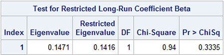
The result of the test is presented as the last part of the printed output (Output 13.10). The hypothesis is accepted (p = .33).

Output 13.10: Test Result when Testing One Restriction

The estimated β parameters (Output 13.11) include only one estimated number because of the normalization. That is the intercept. It is estimated as .12, which is close to zero according to intuition.

Output 13.11: Estimated β Parameters without a Restriction on the Intercept

Tests for Two Restrictions on the β Parameters

In Program 13.4, the further restriction that the intercept is zero is also included. In this situation, the matrix H has just a single column.

Program 13.4: Testing Two Hypotheses on the β Parameters

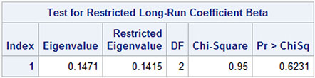
The test accepts the hypothesis. See Output 13.12. The test is a chi-square test on an eigenvalue in a matrix. Note that the degrees of freedom number equals the number of restrictions to the parameters in this test. The mathematics behind this test is rather involved and does not follow the usual lines of statistical theory.

Output 13.12: Test Result When Testing Two Restrictions

Estimated α Parameters under the Restrictions

The output also includes the estimated α parameters when the restrictions are imposed. They are reported in Output 13.13 as an output part entitled “Cointegration Hypothesis Test”. Note that the estimation results printed in the output element entitled “Estimation,” which is generated by Program 13.3 or Program 13.4, are for the error correction model with no restrictions imposed.

Output 13.13: Estimated Parameters under the Restrictions of Program 13.4

The β parameters are simply equal +1, −1, and 0 because the long-run relation is restricted to y_t − x_t ≈ 0, where y_t is the Ohio price and x_t is the Pennsylvania price. The last β coefficient is reported as 0 for the intercept, which is excluded from the relation. An intercept corresponds to a variable that has the constant value 1.

With this restriction on the β parameters, only the α parameters remain free. They are also reported as a part of Output 13.13. The parameter α₁ is close to −1, and α₂ is close to −.5. In the next section, the hypothesis α₁ = 2α₂ is tested because PROC VARMAX also supports testing on the α parameters.

Tests of Hypotheses on the α Parameters by PROC VARMAX

For the α parameters, the hypothesis is stated in a similar way by a matrix J. In the simple situation of a bivariate series as in the Ohio and Pennsylvania potato price example, a restriction on the two-dimensional α vector leaves only a single free parameter. The situation is simply

$$\alpha =\left(\begin{array}{c}{\alpha }_1\\ {\alpha }_2\end{array}\right)=J\Psi =\left(\begin{array}{c}{j}_1\\ j_2\end{array}\right)\left({\psi }_{11}\right)$$

In the conclusion of the previous section, the hypothesis α₁ = 2α₂ was stated as a plausible hypothesis for the price example in two American states. This hypothesis corresponds to the matrix J

$$J=\left(\begin{array}{c}1\\ 0.5\end{array}\right)$$

which gives

$$\alpha =\left(\begin{array}{c}{\alpha }_1\\ {\alpha }_2\end{array}\right)=J\psi =\left(\begin{array}{c}1\\ .5\end{array}\right)\left({\psi }_1\right)=\left(\begin{array}{c}{\psi }_1\\ \raisebox{1ex}{${\psi }_1$}\!\left/ \!\raisebox{-1ex}{$2$}\right.\end{array}\right)$$

This formulation meets the hypothesis α₁ = 2α₂ as α₁ = ψ₁ and α₂ = ψ₁/2.

The hypothesis on the α parameters is tested by Program 13.5. The J matrix is just added to the COINTEG statement in Program 13.5. The COINTEG statement is otherwise unchanged.

Program 13.5: Testing a Restriction on the α Parameters

The test for the α parameters is performed independent of the test on the β parameters. A test for the combined hypothesis is not presented. This means that the output from Program 13.5 in almost all aspects is equivalent to the output from Program 13.4. The only difference is the last part, which is devoted to the restriction on the α parameters. This part is presented in Output 13.14.

Output 13.14: Test Results for the α Parameters

The J matrix is printed as a part of the output from Program 13.5 to ensure that the setup is correct. Both the α parameters and the β parameters are estimated under the restriction on the α parameters but taking no notice of the restriction on the β parameters. The estimated β parameters are very close to the values (1 −1 0). This result is in line with the hypothesis accepted in the previous section. The estimated α parameters of course meet the restriction α₁ = 2α₂ because the hypothesis was formulated in accordance with an observed fact in the series. The hypothesis on the α parameters is accepted for that reason with a p-value as high as .94.

The TEST Statement for Hypotheses on the α Parameters

The hypotheses on the α parameters can alternatively be tested by the TEST statement in PROC VARMAX. This feature is new in SAS/ETS 14.1. Note that the TEST statement does not support hypotheses on the β parameters.

The hypothesis on the α parameters is easily stated in Program 13.6 as a linear restriction α₁ = 2α₂ in the TEST statement. The notation for the restrictions in the TEST statement has the same form as in earlier chapters for testing (for instance, autoregressive parameters, etc., in VARMA models).

Note that Program 13.6 does not include the insignificant constant β₀ in the long-run equation, because the option ECTREND is left out in the COINTEG statement, but the other β parameters are estimated and printed subject to the normalization β₁ = 1.

Program 13.6: Testing Restrictions on the α Parameters

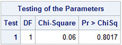
The hypothesis is clearly accepted p = .80. See Output 13.15. The precise test result is not exactly as in Output 13.14 because the test statistics have different definitions. The test using the J matrix is a type of likelihood ratio test while the TEST statement gives a Wald test. These test definitions are only asymptotically equivalent.

Output 13.15: Test Results

The RESTRICT Statement for the β Parameters

The hypothesis α₁ = 2α₂ can also be tested in the model with restrictions on the β parameters. This is possible because the β parameters are allowed in the RESTRICT statement. As noted before, the β parameters are not allowed in the TEST statement.

Program 13.7 gives the code for testing the hypothesis α₁ = 2α₂ in the model where β₁ = 1 and β₂ = − 1. Note that the normalizing option NORMALIZE=OHIO for β₁ = 1 is left out in this application. The NORMALIZE option is not allowed if the β parameters are restricted in the RESTRICT statement.

Program 13.7: Restricting the β Parameters by a RESTRICT Statement

The hypothesis is again clearly accepted (see Output 13.16), having almost the same p-value as in Output 13.14 and Output 13.15.

Output 13.16: Test Results

The INITIAL statement in Program 13.7 is necessary because the estimation otherwise fails. It is often seen that the estimation in complicated multivariate time series models finds local maxima of the likelihood function and not a global maximum. In other situations, the algorithm finds a maximum outside the allowed parameter space. Such convergence problems often occur for moving average parameters and for α parameters in error correction models.

If the INITIAL statement is left out of Program 13.7, the estimation gives positive α parameters, and the αβ^T matrix is totally different from the αβ^T matrix reported in Output 13.5 for completely unrestricted estimation. Note that the β parameters are also stated in the INITIAL statement, even if it seems unnecessary when they are stated in the RESTRICT statement. But the INITIAL statement is neglected if the β parameters are not mentioned in the INITIAL statement.

The actual numbers in the INITIAL statement for the β parameters are of course the values for the restriction. The numbers for the α parameters are taken from Output 13.3, which gave the estimates in the model without restrictions on the β parameters.

The numbers in the INITIAL statement in Program 13.7 are stated in two ways. The initial values for the α parameters are coded individually for α₁ and α₂. In this example, the rank of the β matrix is 1, and the number of columns of the α matrix is also 1. The second index in the notation ALPHA(1,1), the column number, is therefore simply 1 in this example. The β parameters are stated in a matrix notation the same way as the notation for the H and J matrices.

Restrictions on Both α Parameters and β Parameters

In Program 13.8, the restrictions on both the α parameters and the β parameters are simultaneously applied. In this way, a final model for this particular data example is found. In this situation, the INITIAL statement is also necessary. In Program 13.8, the initial values are simply the same as in Program 13.7, even if they are not in line with the restrictions on the α parameters.

Program 13.8: Restrictions on both α Parameters and β Parameters

The resulting α parameters and β parameters are printed as shown in Output 13.17. In Output 13.17, the table, which includes standard deviations for the α parameters, is printed. Because of the restriction α₁ = 2α₂, the standard deviations for α₁ and α₂ are equal.

Output 13.17: Estimated α Parameters and β Parameters

The resulting αβ^T matrix from Program 13.8 is printed; Output 13.18. This estimated αβ^T matrix is almost the same as for the first estimation shown in Output 13.5 with no restrictions at all on the parameters and also allowing for a constant term β₀ in the long-run equation.

Output 13.18: The αβ^T Matrix

In this final model, two restrictions are applied. The restriction on the α parameters is tested by a Lagrange multiplier test. See Output 13.19. The restriction is accepted by this test with p = .88. The large p-value is natural because the hypothesis is formulated as a relation almost established in the unrestricted estimation.

Output 13.19: Tests for the Restrictions

Properties of the Final Model

In the following, both the hypothesis on the α parameters and the β parameters are included in the model, and the free α parameter is set to .96 as in Output 13.18. The model is now written as

y_t =  y_t−1 − .96( y_t−1 − x_t−1) + ...

for the Ohio price series and

x_t =  x_t−1 − .48( y_t−1 − x_t−1 ) + ...

for the Pennsylvania price series.

The correction in the Ohio series nearly perfectly corrects for the observed difference in the two price series at time t − 1. The correction would be perfect if the coefficient was 1 instead of .96. The correction in the Pennsylvania series, however, is in the “wrong” direction as its individual contribution multiplies the observed difference y_t−1 − x_t−1 by .48. The combined effect of the model is that the difference y_t−1 − x_t−1 is reduced by the factor .52.

Moreover, autoregressive parameters are estimated for the differenced series in order to formulate a model with residuals without autocorrelation. In error correction models, the autoregressive parameters are, however, of only minor importance compared with the error correction part.

Conclusion

It is possible to argue for error correction models based on pure intuition. Error correction models allow two or more series to behave according to a stable linear relation, an equilibrium. If the series for some reason comes away from this stable relation, the error correction mechanism tries to lead all series toward the relation again.

The underlying theory tells how to estimate the parameters in this refined model and how to test for hypotheses involving these parameters. PROC VARMAX makes all available. You have learned how easy it is to perform such an analysis, seeing how PROC VARMAX works in a simple example of two series of potato prices in two neighboring U.S. states that, of course, should be parallel in this regard.