
19 Mechanics of Statistics
Overview
This chapter is an essay on fitting for those of you who are mechanically inclined. If you have any talent for imagining how springs and tire pumps work, you can put it to work here in a fantasy in which all the statistical methods are visualized in simple mechanical terms.
The goal is to not only remember how statistics works, but also train your intuition so that you are prepared for new statistical issues.
Here is an illuminating trick that helps you understand and remember how statistical fits really work. It involves pretending that statistical fitting is performed by machines. If we can figure out the right machines and visualize how they behave, we can reconstruct all of statistics by putting together these simple machines into arrangements appropriate to the situation. We need only two machines of fit, the spring for fitting continuous normal responses and the pressure cylinder for fitting categorical responses.
Readers interested in this approach should consult Farebrother (2002), who covers physical models of statistical concepts extensively.
Chapter Contents
Springs for Continuous Responses
Effect of Sample Size Significance
Effect of Error Variance on Significance
Experimental Design’s Effect on Significance
Summary: Significance and Power
Mechanics of Fit for Categorical Responses
How Do Pressure Cylinders Behave?
One-Way Layout for Categorical Data
Springs for Continuous Responses
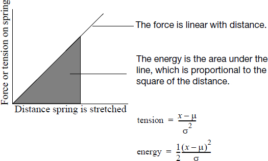
How does a spring behave? As you stretch the spring, the tension increases linearly with distance. The energy that you need to pull a spring a given distance is the integral of the force over the distance, which is proportional to the square of the distance.
Take 1/σ2 as the measure of how stiff a spring is. Then the graph and equations for the spring are as shown in Figure 19.1.
Figure 19.1 Behavior of Springs
In this way, springs help us visualize least squares fits. They also help us do maximum likelihood fits when the response has a normal distribution.
The formula for the log of the density of a normal distribution is identical to the formula for energy of a spring centered at the mean, with a spring constant equal to the reciprocal of the variance. A spring stores and yields energy in exactly the way that normal deviations get and give log-likelihood. So, maximum likelihood is equivalent to least squares, which is equivalent to minimizing energy in springs.
Fitting a Mean
How do you fit a mean by least squares? Imagine stretching springs between the data points and the line of fit (see Figure 19.2). Then you move the line of fit around until the forces acting on it from the springs balance. That will be the point of minimum energy in the springs. For every minimization problem, there is an equivalent balancing (or orthogonality) problem, in which the forces (tensions, relative distances, residuals) add up to zero.
Figure 19.2 Fitting a Mean by Springs

Testing a Hypothesis
Suppose that you want to test a hypothesis that the mean is some value. You would force the line of fit to be that value and measure how much more energy you had to add to the springs (how much more the sum of squared residuals was) to constrain the line of fit. This is the sum of squares that is the main ingredient of the F-test. To test that the mean is (not) the same as a given value, find out how hard it is to move it there (see Figure 19.3).
Figure 19.3 Compare a Mean to a Given Value

One-Way Layout
If you want to fit several means, you can do so by balancing a line of fit with springs for each group. To test that the means are the same, you force the lines of fit to be the same, so that they balance as a single line. You also measure how much energy you had to add to the springs to do this (how much greater the sum of squared residuals was). See Figure 19.4.
Figure 19.4 Means and the One-Way Analysis of Variance

Effect of Sample Size Significance
When you have a larger sample, there are more springs holding on to each mean estimate, and it is harder to pull them together. Larger samples lead to a greater energy expense (sum of squares) to test that the means are equal. The spring examples in Figure 19.5 show how sample size affects the sensitivity of the hypothesis test.
Figure 19.5 A Larger Sample Helps Make Hypothesis Tests More Sensitive

Effect of Error Variance on Significance
The spring constant is the reciprocal of the variance. Thus, if the residual error variance is small, the spring constant is bigger, the springs are stronger, it takes more energy to bring the means together, and the test is therefore more significant. The springs in Figure 19.6 illustrate the effect of variance size.
Figure 19.6 Reduced Residual Error Variance Makes Hypothesis Tests More Sensitive

Experimental Design’s Effect on Significance
If you have two groups, how do you arrange the points between the two groups to maximize the sensitivity of the test that the means are equal? Suppose that you have two sets of points loading two lines of fit, as in the one-way layout shown previously in Figure 19.4. The test that the true means are equal is done by measuring how much energy it takes to force the two lines together.
Suppose that one line of fit is suspended by a lot more points than the other. The line of fit that is suspended by few points will be easily movable and can be stretched to the other mean without much energy expenditure. The lines of fit would be more strongly separated if you had more points on this loosely sprung side, even at the expense of having fewer points on the more tightly sprung side. It turns out that to maximize the sensitivity of the test for a given number of observations, it is best to allocate points in equal numbers between the two groups. In this way, both means are equally tight, and the effort to bring the two lines of fit together is maximized.
So the power of the test is maximized in a statistical sense by a balanced design, as illustrated in Figure 19.7.
Figure 19.7 Design of Experiments

Simple Regression
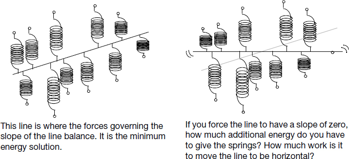
If you want to fit a regression line through a set of points, you fasten springs between the data points and the line of fit, such that the springs stay vertical. Then let the line be free so that the forces of the springs on the line balance, both vertically and rotationally (see Figure 19.8). This is the least squares regression fit.
Figure 19.8 Fitting a Regression Line with Springs

If you want to test that the slope is zero, you force the line to be horizontal so that you’re just fitting a mean and measure how much energy it took to constrain the line (the sum of squares due to regression) (see Figure 19.9).
Figure 19.9 Testing the Slope Parameter for the Regression Line
Leverage
If most of the points that are suspending the line are near the middle, then the line can be rotated without much effort to change the slope within a given energy budget. If most of the points are near the end, the slope of the line of fit is pinned down with greatest resistance to force. That is the idea of leverage in a regression model. Imagine trying to force the line to have a different slope. Look at Figure 19.10 and decide which line would be easier to twist.
Figure 19.10 Leverage with Springs

Multiple Regression
The same idea works for fitting a response to two regressors; the difference is that the springs are attached to a plane rather than a line. Estimation is done by adjusting the plane so that it balances in each way. Testing is done by constraining the plane.
Figure 19.11 Three-Dimensional Plot of Two Regressors and Fitted Plane

Summary: Significance and Power
Suppose that you want a stronger (more significant) fit, in which the line of fit is suspended more tightly. You must either have stiffer springs (have smaller variance in error), use more data (have more points to hang springs from), or move your points farther out on both ends of the x-axis (more leverage). The power of a test is how likely it is that you will be unable to move the line of fit given a certain energy budget (sum of squares) determined by the significance level.
Mechanics of Fit for Categorical Responses
Just as springs are analogous to least squares fits, gas pressure cylinders are analogous to maximum likelihood fits for categorical responses (see Figure 19.12).
How Do Pressure Cylinders Behave?
Using Boyle’s law of gases (pressure times volume is constant), the pressure in a gas cylinder is proportional to the reciprocal of the distance from the bottom of the cylinder to the piston. The energy is the force integrated over the distance (starting from a distance, p, of 1), which turns out to be –log(p).
Figure 19.12 Gas Pressure Cylinders Equate –log(probability) to Energy

Now that you know how pressure cylinders work, start thinking of the distance from the bottom of the cylinder to the piston as the probability that some statistical model attributes to some response. The height of 1 means no stored energy, no surprise, a probability of 1. The height of zero means infinite stored energy, an impossibility, a probability of zero.
When stretching springs, we measured energy by how much work it took to pull a spring, which turned out to be the square of the distance. Now we measure energy by how much work it takes to push a piston from distance 1 to distance p, which turns out to be –log(p), the logarithm of the probability. We used the logarithm of the probability before in categorical problems when we were doing maximum likelihood. The maximum likelihood method estimates the response probabilities so as to minimize the sum of the negative logarithms of the probability attributed to the responses that actually occurred. This is the same as minimizing the energy in gas pressure cylinders, as illustrated in Figure 19.13.
Figure 19.13 Gas Pressure Cylinders Equate –log(probability) to Energy

Estimating Probabilities
Now we want to estimate the probabilities by minimizing the energy stored in pressure cylinders. First, we need to build a partitioned frame with a compartment for each response category and add the constraint that the sum of the heights of the partitions is 1. We will move the partitions around so that the compartments for each response category can get bigger or smaller (see Figure 19.14).
For each observation on the categorical response, put a pressure cylinder into the compartment for that response. After you have all the pressure cylinders in the compartments, start moving the partitions around until the forces acting on the partitions balance out. This will be the solution to minimize the energy stored in the cylinders. It turns out that the solution for the minimization is to make the partition sizes proportional to the number of pressure cylinders in each compartment.
For example, suppose a survey asked 13 people what brand of car they preferred. Five people chose Asian, two chose European, and six chose American brands. Then you would stuff the pressure cylinders into the frame as in Figure 19.14, and the partition sizes that would balance the forces work out to 5/13, 2/13, and 6/13, which sum to 1.
To test that the true probabilities are some specific values, you move the partitions to those values and measure how much energy you had to add to the cylinders.
Figure 19.14 Gas Pressure Cylinders Estimate Probabilities for a Categorical Response

One-Way Layout for Categorical Data
If you have different groups, you can fit a different response probability to each group. The forces acting on the partitions balance independently for each group. The plot shown in Figure 19.15 (which should remind you of a mosaic plot) helps maintain the visualization of pressure compartments. As an alternative to pressure cylinders, you can visualize with free gas in each cell.
Figure 19.15 Gas Pressure Cylinder Estimate Probabilities for a Categorical Response

How do you test the hypothesis that the true rates are the same in each group and that the observed differences can be attributed to random variation? You just move the partitions so that they are in the position corresponding to the ungrouped population and measure how much more energy you had to add to the gas-pressure system to force the partitions to be in the same positions.
Figure 19.16 shows the three kinds of results you can encounter, corresponding to perfect fit, significant difference, and nonsignificant difference. To the observer, the issue is whether knowing which group you are in will tell you which response level you will have. When the fit is near perfect, you know with near certainty. When the fit is intermediate, you have more information if you know the group you are in. When the fit is inconsequential, knowing which group you are in doesn’t matter. To a statistician, though, what is interesting is how firmly the partitions are held by the gases, how much energy it would take to move the partitions, and what consequences would result from removing boundaries between samples and treating it as one big sample.
Figure 19.16 Degrees of Fit

Logistic Regression
Logistic regression is the fitting of probabilities over a categorical response to a continuous regressor. Logistic regression can also be visualized with pressure cylinders (see Figure 19.17). The difference with contingency tables is that the partitions change the probability as a continuous function of the x-axis. The distance between lines is the probability for one of the responses. The distances sum to a probability of 1. Figure 19.18 shows what weak and strong relationships look like.
Figure 19.17 Logistic Regression as the Balance of Cylinder Forces

Figure 19.18 Strengths of Logistic Relationships
