CHAPTER 9

Nonlinear Regression Models

Chapter 9 Preview

When you have completed reading this chapter you will be able to:

• Address nonlinearities with linear least squares regression.
• Estimate a nonlinear regression (four different nonlinear regressions).
• Know when it may be reasonable to use a nonlinear regression model.
• Identify common uses of nonlinear regressions.
• Interpret the results from an estimate of a nonlinear model.

Introduction

All of the regression models you have looked at thus far have been linear. Some have had one independent variable, while others have had several independent variables, but all have been linear. Linear functions appear to work very well in many situations. However, cases do arise in which nonlinear models are called for. The real world does not always present you with linear (i.e., straight-line) relationships.

In some situations, the economic/business theory underlying a relationship may lead you to expect a nonlinear relationship. Examples of such real world cases include the U-shaped average cost functions and S-shaped production functions, both of which are caused by the existence of the law of variable proportions or diminishing marginal returns. Profit and revenue functions often increase at a decreasing rate and then decline, shaped somewhat like an inverted-U(⋂).

Earlier, you learned that plotting data in a scattergram before doing a regression analysis can be helpful. Among other things, this may help us decide on the appropriate form for the model. Perhaps some nonlinear form would appear more consistent with the data than would a linear function.

Quadratic Functions

Look at the two graphs in Figure 9.1. The data for the scattergrams depicted in each graph are listed to the right of the graphs. In the upper graph, the 10 observations appear to form a U-shaped function such as what you might expect of an average variable cost curve. The lower scattergram suggests a function that increases at a decreasing rate and then eventually declines (like an upside-down bowl placed on a table). Clearly, a linear function would not fit either set of data very well. This lack of a linear fit is illustrated by the inclusion of the OLS linear regression line in each graph. In neither case does the (linear) regression line offer a close fit for the data.

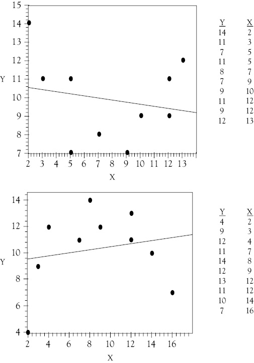
Figure 9.1 Quadratic functions. Scattergrams of data that should be fit with quadratic functions

These scattergrams are indicative of quadratic functions, that is, functions in which X2 appears as an independent variable. But most regression programs are designed for linear problems. Is it possible to use such programs to estimate this type of function? The answer is “yes” and the technique for doing so is surprisingly simple.

You need only define a new variable to be the square of X. Suppose that you use Z. Then Z = X2. You can now estimate a multiple linear regression model of Y as a function of X and Z, which may be expressed as:

Y = a + b1X + b2Z

This is a function that is linear in the variables X and Z.

Estimating a function such as this for the data in the upper graph of Figure 9.1, you get:

Y = 18.26 – 2.71X + 0.17Z

But remember that Z = X². Rewriting the function in terms of Y, X, and X², you have:

Y = 18.26 – 2.71X + 0.17X2

This is a quadratic function in X and has the U-shape you would expect to fit the scattergram (see Figure 9.2).

The data in the lower graph in Figure 9.1 also appear to be quadratic, but this time the function at first goes up and then down (rather than vice versa, as in the previous case). Even though the curvature of this data is an upside-down U-shape, you can use the same technique. Again let Z = X2 and estimate:

Y = a + b1X + b2Z

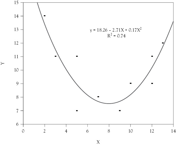
Figure 9.2 A nonlinear regression result. The regression line in this case is nonlinear because a quadratic (squared) term has been added to the regression estimate

This time you expect the sign of bl to be positive and the sign of b2 to be negative (The opposite was true in the previous case). The regression results are:

Y = 1.73 + 2.49X – 0.14Z

Substituting X2 for Z, you have:

Y = 1.73 + 2.49X – 0.14X2

This function would have the inverted U-shape that the scattergram of the data would suggest (see Figure 9.3).

Cubic Functions

How would you handle situations in which the perceived curve exhibited by a set of data has more than a single curvature? Is OLS regression able to model such data? Yes, you can model data with a double curvature but the technique will require the use of a cubed term. Now take a look at the scattergrams and data shown in Figure 9.4. You can see that a linear function would not fit either of these data sets very well. The data in the upper graph might represent a cost function, while that in the lower graph may be a production function. Both are polynomials, but they are cubic functions, rather than quadratic functions.

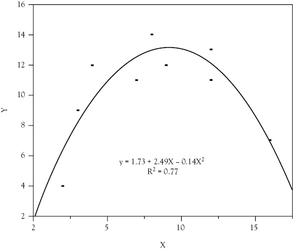
Figure 9.3 A second nonlinear regression result. The regression line in this case is again nonlinear because a quadratic (squared) term has been added to the regression estimate. However, in this regression, the squared term has a negative coefficient and the resulting regression line is in the form of an upside-down U-shape

To estimate these cubic functions using a multiple linear regression model, you can let Z = X2 and W = X3. The linear function is then:

Y = a + b1X + b2Z + b3W

Using the data in the lower graph in Figure 9.4, you get the following regression equation:

Y = 1.02 + 1.63X – 0.31Z + 0.021W

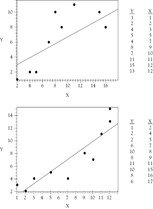
Figure 9.4 Cubic functions. These two data sets should be fit with cubic functions. The OLS linear functions are shown in the scattergrams and are seen to not fit the data well

Substituting X2 for Z and X3 for W, you get:

Y = 1.02 + 1.63X – 0.31X2 + 0.021X3

You can see this result in Figure 9.5.1

The t-ratios are fairly low even though the function fits the data pretty well which might be puzzling. The main reason is related to the small number of data points relative to the number of variables. You would rarely estimate a regression analysis with just 10 observations, especially when using 3 independent variables. However, using just 10 observations is helpful in learning the concepts.

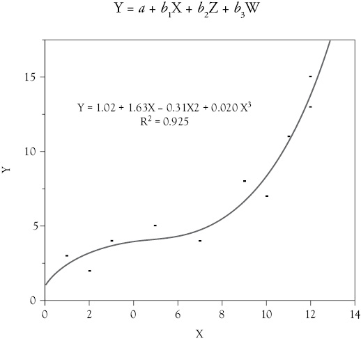
Figure 9.5 Cubic functions. This cubic form regression is fit with the data from the lower graph in Figure 9.4

You see that the upper scattergram in Figure 9.4 also appears to have two turning points: one near X = 6 and the other in the vicinity of X = 11. This indicates that a cubic function might again be appropriate. You again let Z = X2 and W = X3. The linear function is then:

Y = a + b1X + b2Z + b3W

Using the data in the upper graph in Figure 9.4, you get the following regression equation:

Y = 1.03 – 0.80X + 0.33Z – 0.016W

Substituting X2 for Z and X3 for W, you get:

Y = 1.03 – 0.80X + 0.33X2 – 0.016X3

You can see this result in Figure 9.6.

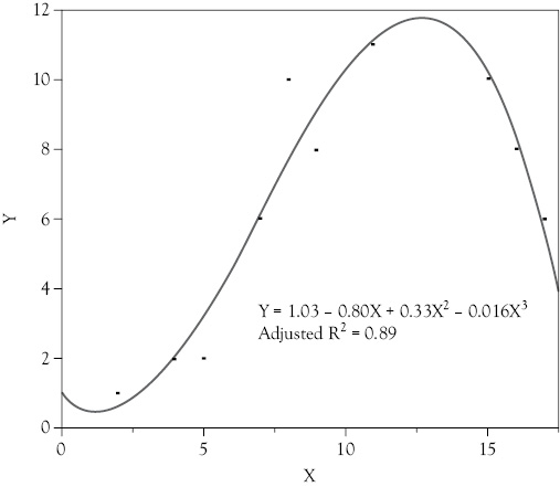
Figure 9.6 Cubic functions. This cubic form regression is fit with the data from the upper graph in Figure 9.4

Reciprocal Functions

Now look at the scattergrams and data in Figure 9.7. In the upper graph, you see that the Y values fall rapidly as X increases at first, but then as X continues to increase, the Y value seems to level off. The lower graph is similar except that, as X increases, at first Y increases rapidly but seems to reach a plateau. Now, consider using a reciprocal transformation to estimate each of these sets of data; that is, use 1/X rather than X as the independent variable.

You can let U = 1/X and proceed to estimate the function: Y = a + bU. Using the data from the upper graph in Figure 9.7, the regression equation is:

Y = 5.91 + 16.52U

Substituting 1/X for U, you have:

Y = 5.91 + 16.52(1/X)

For this function, as X increases 1/X decreases. As a result, this function approaches the value of the constant term of the regression (a = 5.91) from above as X gets large as you see in Figure 9.8.

Using the same approach for the data in the lower graph in Figure 9.7, the regression results yield:

Y = 12.38 – 11.53(1/X)

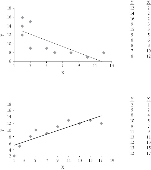
Figure 9.7 Reciprocal functions. The data sets shown here can be fit well with reciprocal functions. The OLS linear functions are shown on each scattergram and are seen to not fit the data well in either case

For this function, as X increases, this function also approaches the value of the constant term of the regression (a = 12.38), but from below rather than above. You can see this graphically in Figure 9.9.

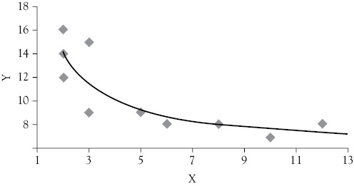
Figure 9.8 A reciprocal function. This reciprocal form regression is fit with the data from the upper graph in Figure 9.7

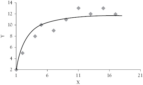
Figure 9.9 A second reciprocal function. This reciprocal form regression is fit with the data from the lower graph in Figure 9.7

Multiplicative Functions2

The final type of nonlinear function included here involves a double-log transformation. This allows you to use a multiple linear regression program to estimate the following functional form:

Y = AX1 b1X2 b2

Functions of this type are called power functions or multiplicative functions. The most common of these functions is the Cobb-Douglas production function. The general form for such a function is:

Q = ALb1Kb2

where, Q is output, L is labor input, and K is capital. This example uses just L and K but each of these could have subcomponents so there could be many Ls and many Ks.

These functions are clearly nonlinear, so you must use some transformation to get them into a linear form. If you take the logarithms of both sides of the equation, you have:

Y = AX1b1X2b2

lnY = lnA + bllnX1 + b2lnX2

where ln represents the natural logarithm. Now, you can let W = InY, a = lnA, U = lnX1, and V = lnX2. The function is now linear in W, U, and V, as shown below:

W = a + blU + b2V

A function such as this can be estimated using a standard multiple regression program. For example, consider the data in Table 9.1. Y is the dependent variable, X1 and X2 are independent variables, and you would like to estimate the following function:

Y = AX1b2X2b2

Using Excel, you can easily find the natural logarithms of all three variables (W = lnY, U = lnXl, and V = lnX2). These values are also shown in Table 9.1.3

Using the natural logarithms as the variables, you estimate the following multiple linear regression:

W = 2.402 + 0.407U + 0.474V

Table 9.1 Data for a power function

Y	X	X	W = lnY	U = lnX	V = InX
39.73	1	15	3.682	0.000	2.708
55.37	8	5	4.014	2.079	1.609
41.59	2	9	3.728	0.693	2.197
69.75	6	10	4.245	1.792	2.303
52.25	4	8	3.956	1.386	2.079
87.31	10	11	4.469	2.303	2.398
52.37	5	7	3.958	1.609	1.946
96.60	12	12	4.571	2.485	2.485
66.60	7	8	4.199	1.946	2.079
92.83	9	13	4.531	2.197	2.565

Making the appropriate substitutions for W, U, and V, you have:

lnY = 2.402 + 0.407lnX1 + 0.474lnX2

Taking the antilogarithm of the equation, you obtain:

Y = (e2.402)X1.407 X2.474

where e represents the Naperian number (2.7183), which is the base for natural logarithms. Thus,

Y = (2.71832.402)X1.407 X2.474

Y = 11.04X1.407 X2.474

Converting 2.71832.402 to 11.04 is easily done using the EXP function in Excel. You see that this fairly complex-looking function can be estimated with relative ease using the power of multiple regression and the logarithmic transformation. Power or multiplicative functions, such as this, are not only commonly found as production functions but are also sometimes used for demand functions.

Even though the basic regression model is designed to estimate linear relationships, nonlinear models can be estimated by using various transformations of the variables. Polynomial functions can be estimated by using second, third, and/or higher powers of one or more of the independent variables. Logarithmic and reciprocal transformations are also commonly used.

What You Have Learned in Chapter 9

• How nonlinearities can be addressed with linear least squares regression.
• To estimate a nonlinear regression (four different nonlinear regressions).
• To recognize when it may be reasonable to use a nonlinear regression model.
• To be familiar with common uses of nonlinear regressions.
• How to interpret the results of an estimate of a nonlinear model.

---