CHAPTER 11

The Formal Ordinary Least Squares (OLS) Regression Model

Chapter 11 Preview

When you have completed reading this chapter you will be able to:

• Understand how software packages calculate the least squares regression estimate.
• Know the rule that every software package uses to choose the best regression estimate.
• Understand how R-square is calculated.
• Know how to use the Akaike Information Criterion (AIC) to choose independent variables correctly.
• Know how to use the Schwartz Criterion (SC) to choose independent variables correctly.

Introduction

You now have a good understanding of applied regression analysis. You can now do simple and sophisticated forms of regression. You know how to evaluate and interpret regression models. Some of you may be interested in the mathematics that forms the foundation of ordinary least squares (OLS) regression. You will get a start on this formal understanding as you read this chapter.

A Formal Approach to the OLS Model

In mathematical notation, the true simple linear regression is expressed as:

Yi = α + β Xi + εi

where

Yi = the value of the dependent variable for the ith observation

Xi = the value of the independent variable for the ith observation

εi = the value of the error for the ith observation

α = intercept of the true regression line on the vertical, or Y, axis.

(This may also be called the constant term in regression software.)

β = slope of the true regression line

Normally, the data do not follow an exactly linear relationship. In the scattergram in Figure 11.1, for example, it is impossible to draw one straight line that will go through all the points. The method of OLS is a way of determining an equation for a straight line that best (according to the least squares criterion) represents the relationship inherent in the data points of the scatter diagram. The general form of this estimated linear function may be stated as:

YiE = aE + bE Xi

where aE and bE are the calculated (or estimated) values of the intercept and the slope of the line, respectively. YiE is the calculated value for the dependent variable that is associated with the independent variable Xi.

Since the (YiE) values are all located on the “calculated” straight line, the actual Yi values will, in most cases, differ from your calculated (YiE) values by a residual amount, which are denoted as ei. (These residuals may also be referred to as deviations, or errors.). Mathematically, this can be expressed as:1

Yi – YiE = ei

and thus,

Yi = YiE + ei

Further, since you have defined YiE = aE +bEXi, this expression may be written as:

Yi = aE + bEXi + ei

There are at least two reasons for the existence of the residual (ei) in the previous equation:

1. It is impossible to know and have data for all the factors that influence the behavior of the dependent variable
2. There are errors in observation and measurement of economic data.

Thus, it is normally impossible for one straight line to pass through all the points on the scatter diagram, and it becomes necessary to specify a condition that the line must satisfy to make the line in some sense better than any of the other lines that could be drawn through the scatter diagram. The OLS condition can be stated as follows:

The line must minimize the sum of the squared vertical distances between each point on the scatter diagram and the line.

In terms of Figure 11.1, the line must minimize the sum of the squared residuals, that is, minimize ∑e2.

The linear relationship, or line, that satisfies this condition is called an OLS regression line. The expression for the sum of the squared vertical distances is:

∑ei2 = ∑(Yi –YiE)2

∑ei2 = ∑(Yi – aE – bEXi)2

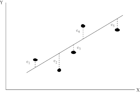
Figure 11.1 The OLS regression line for Y as a function of X. Residuals (or deviations or errors) between each point and the regression line are labeled ei

where each expression is summed over the n observations of the data, that is, for i = 1 to i = n. In this expression, the a_E (the Y intercept) and b_E (the slope) are the unknowns, or variables. Given this equation, the objective is to obtain expressions, or normal equations, as they are called by statisticians, for a_E and bE that will result in the minimization of ∑ ei2.

The normal equations are:2

bE = (∑Y iXi - nYMXM) ÷ (∑ Xi2 - nXM2)

aE = YM - bE XM

where YM and XM are the means of Y and X, respectively.

These two equations can then be used to estimate the slope and intercept, respectively, of the OLS regression function. Every software package that calculates OLS regression results uses these normal equations. Most of you have a calculator that does a trend and/or a bivariate regression. These normal equations are the basis for those functions in your calculator. These same normal equations are the basis of regression models estimated by every software package.

As a matter of course, you would not use these normal equations to estimate the intercept and slope terms for regression problems manually. Today, computers and appropriate software are available to everyone seriously interested in performing regression analyses. Statistical and forecasting software such as ForecastX, SAS, and SPSS, all provide good regression procedures. As you have seen, even Microsoft Excel has the capacity to calculate regression (albeit without producing some of the summary statistics needed for business use).

The Development of R-square

You learned about the coefficient of determination (R-squared) and about how it can be interpreted as the percentage of the variation (i.e., “up and down movement”) in a dependent variable that can be explained by a regression model. Now that you know what R-square is, let us consider how this measure can be developed.

The total variation in Y is measured as the sum of the squared deviations of each Y value from the mean value of Y.

Figure 11.2 will help you to see why this summary statistic is used to measure the variation in Y. The large dot represents a single observation on two variables, X and Y. In Figure 11.2, you can see the following:

• Total variation = distance between the data point (Yi) and the reference line at the mean of Y ().
• Explained variation = distance between the reference line at the mean of Y () and the regression estimate ()
• Unexplained variation = distance between the data point (Yi ) and the regression line ().

In Figure 11.2, the horizontal line drawn at the mean value for Y (i.e., YM) is called the reference line. The single data point shown is not on the regression estimated regression line. The amount by which the observation differs from the mean of Y is shown by the distance labeled “total variation.”

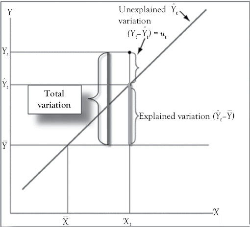
Figure 11.2 Partitioning the variation in Y. The total variation in the dependent variable (Y) can be separated into two components: Variation that is explained by the regression model and variation that is unexplained

Part of that total variation in Y is explained by the regression model, but part is unexplained. Let’s look at the latter. The difference between each observed value of Y and the value of Y determined by the regression equation is a residual variation that has not been explained or accounted for (see the segment labeled “unexplained variation”).

The part of the total variation in Y that is explained by the regression model is called the “explained variation.” For each observation, the explained variation can be represented by the distance between the value estimated by the regression line () and the mean of Y ().

Does it not make sense that the sum of the “explained” plus the “unexplained” variations should equal the total variation? Note that the distance labeled “total variation” in Figure 11.2 is the sum of the “explained” and “unexplained” variations. This makes it possible to measure the total variation in Y and explain how much of that variation is accounted for by the estimated regression model.

This brings us back to the coefficient of determination (R2). Recall that R-square is the percentage of the total variation in Y that is explained by the regression equation. Thus, R-square must be the ratio of the explained variation in Y to the total variation in Y:

R2 = (Explained variation in Y) ÷ (Total variation in Y)

The Akaike and Schwarz Criteria3

Sometimes the diagnostic tools you have looked at thus far can be contradictory in helping us identify the “best” regression model from among some set of alternatives. This is particularly likely when the various models have different numbers of independent variables. Thus, you sometimes want to consider two other measures that can be helpful in selecting a model.

One such measure calculated in many commercially available software programs is the Akaike information criterion (AIC), which considers both the accuracy of the model and the principle of parsimony (i.e., the concept that fewer independent variables should be preferred to more, other things being equal). The calculation of AIC is mathematically complex but what is important here is to know that it is designed such that lower absolute values are preferred to higher ones. In AIC, as additional independent variables are included in the model the value of AIC will increase unless there is also sufficient new information to increase accuracy enough to offset the penalty for adding new variables. If the absolute value of AIC declines significantly, after adding a new independent variable to the model, accuracy has increased enough after adjustment for the principle of parsimony.

The Schwarz criterion (SC) is quite similar to AIC in its use and interpretation. However, it is very different in its calculation, using Bayesian arguments about the prior probability of the true model to suggest the correct new model. A significantly lower absolute value for SC is preferred to a higher one, just as with AIC. If the absolute value of SC decreases after the addition of a new independent variable, the resulting model is considered superior to the previous one.

Building and Evaluating Three Alternative Models of Miller’s Foods’ Market Share

In this section, you will work through the process of building regression models for the Miller’s Foods’ market share data that you saw earlier in Chapter 7. You will consider three competing models. In the process you also expand on your knowledge of regression modeling by using the AIC and SC criteria.

Scattergrams of Miller’s Foods’ Market Share with Potential Independent Variables

It is a good idea to start your regression modeling by looking at graphic representations of the relationship between the dependent variable and the causal independent variables that are being considered for the model. In this example, you are going to consider price (P), advertising (AD), and an index of competitor’s advertising (CAD) as potential factors influencing Miller’s market share. These scattergrams, in Figure 11.3, only tell part of the story, but they can be a useful first step in getting a feel for the relationships that are involved.

The Statistical Hypotheses

Your hypotheses about these independent variables can be summarized as:

For Price: H0 : β1 ≥ 0; H1 : β1 < 0

Rationale: As price rises, people buy less from Miller’s and share falls.

For Advertising: H0 : β2 ≤ 0; H1 : β1 > 0

Rationale: When advertising increases, sales and share increase as well.

For the competitors’ index of advertising:

H0 : β1 ≥ 0; H1 : β1 < 0

Rationale: As the index rises, competitors are advertising more and Miller’s loses market share.

In each of the advertising scattergrams (see Figures 11.3B and 11.3C) you see visual support for the hypotheses suggested above. However, for the price scattergram (Figure 11.3A), the hypothesis seems incorrect. This is likely due to the fact that you are examining price alone without the two other variables that you know act with it to determine sales.

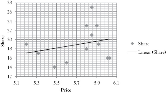
Figure 11.3A Scattergram of Miller’s Foods’ market share with price

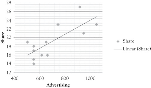
Figure 11.3B Scattergram of Miller’s Foods’ market share with advertising

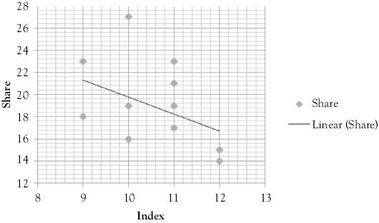
Figure 11.3C Scattergram of Miller’s Foods’ market share with the index of competitor’s advertising

The Three Alternative Models

With three possible independent variables there are many alternative models that you could construct. Consider the following three regression models:

Share = f (Price)

Share = f (Price, Advertising)

Share = f (Price, Advertising, Index)

Rather than show the results for these models in the form of their respective computer printouts they are summarized in Table 11.1. When a number of alternative models are presented, it is a common practice to organize the results in a table such as this to facilitate easy comparison between them.

From the information in Table 11.1, you can perform the five-step evaluation process. First, the signs on all coefficients in all of the models are consistent with our expectations (with the exception of price in the simple regression shown in Model 1), so the models make sense from a theoretical perspective. Second, all of the t-ratios are large enough (with the exception of price in Model 1 and Model 2) to allow us to reject the corresponding null hypotheses. Thus, in general you find statistically significant relationships.

The coefficients of determination vary from a low of 6.58 percent to a high of 81.17 percent. Model 3 has an adjusted R-square of 81.17 percent which means that 81.17 percent of the variation in Miller’s Foods’ market share is explained by variation in price, advertising, and the index of competitors’ advertising.

Table 11.1 Three OLS multiple regression models for Miller’s Foods’ market share

Variable	OLS Model 1	OLS Model 2	OLS Model 3
Intercept	–2.05	17.79	80.01
P	3.67 (0.84)	–1.87 (–0.55)	–8.46 (–3.13)
AD	–	0.02 (3.46)	0.02 (6.40)
CAD	–	–	–2.54 (–3.92)
R-square or Adjusted R-square	6.58%	51.03%	81.17%
Durbin–Watson	0.63	1.39	2.17
Std. Error of Est.	3.91	2.70	1.68
SC	66.62	56.46	43.58
AIC	67.10	56.94	44.06

*Values in parentheses are t-ratios.

The DW statistic for the three models improves as variables are added. For Model 3, the DW statistic of 2.17 indicates possible negative serial correlation, but it is likely not severe enough to be of concern given how large the t-ratios are in Model 3. The DW of 2.17 satisfies Test 2 in Appendix 4D indicating the result is indeterminate. If the calculated DW statistic was between 2 and 2.072, Test 3 would be satisfied indicating no serial correlation.

Finally, you should check the correlation matrix to evaluate the potential of multicollinearity. The correlation matrix for the independent variables is:

	P	AD	CAD
P	1.00
AD	0.47	1.00
CAD	–0.59	–0.09	1.00

None of these correlations among the independent variables indicates the presence of severe multicollinearity.

Note that as each variable is added to the simple regression, the AIC and SC decrease by 10 or more points; this indicates that each variable added is likely to be a correct variable to include in the model.

What You Have Learned in Chapter 11

• You understand how software packages calculate the least squares regression estimate.
• You know the rule that every software package uses to choose the best regression estimate.
• You understand how R2 is calculated.
• You know how to use the AIC and the SC to evaluate regression models correctly.

---