
Chapter 6: Data Tasks Using Hash Table Operations
6.2.1 Two Principal Methods of Subsetting
6.2.2 Simple Data File Subsetting via a Hash Table
6.2.3 Why a Hash Table and Not SQL?
6.2.4 Subsetting with a Twist: Adding a Simple Count
6.3.2 Merging a Join with an Aggregate
6.3.4 DO_OVER Versus FIND + FIND_NEXT
6.4.1 Hash Data Split - Sorted Input
6.4.2 Hash Data Split - Unsorted Input
6.5 Ordering and Grouping Data
6.5.1 Reordering Split Outputs
6.1 Introduction
In Chapters 2-4, we have discussed how the hash object tools can be used to perform hash table operations. In this chapter, in response to a request from the IT users at Bizarro Ball headquarters, we will discuss how the operations can be applied to address a number of common data processing tasks using terminology that they are familiar with. In later chapters in this part we will refocus our efforts on the requirements (and terminology) of the business users.
In particular, we will apply hash table operations to:
● Subset, unduplicate, combine, split, and order data.
● Implement or supplant dynamic data structures, such as arrays, stacks, queues, etc.
● Use hash tables as dynamic storage media to discover certain data properties.
The examples and code snippets in this chapter are kept at the complexity level needed to demonstrate the principle. However, they are complete enough to serve as practical templates for more sophisticated examples found in the next chapters, as well as in the programs used to create the sample data.
Our challenge is to first convince the IT users that the underlying technology and functionality can address their concerns while at the same time meeting all of the business users’ requirements. In the following sections we will lead with terminology that the IT users are most comfortable with and also describe the functionality that the business users are comfortable with. Anyone who has dealt with describing technology solutions knows that IT and business users quite often don’t speak the same language, and so we have to serve as translators.
6.2 Subsetting Data
Subsetting is an act of selecting a subset from one data collection (let us call it A) based on values from another data collection (let us call it B). "Data collection" can be pretty much anything: a flat file, an array, a set of macro variables, etc. Most commonly, the collection A is represented by a SAS data file or its logical equivalent. The collection whose values are used to do the subsetting (B) can take various forms depending on its size and other circumstances. However, it can be assumed without a loss of generality that the values of B are also stored in a SAS data file since the file can be used to generate subsetting code using any lookup technique in the SAS arsenal.
For the benefit of our business users, subsetting data might include something like the example in the case study in Chapter 12 where our subset is defined using the data in the Pitches data set (all the data where the first two pitches are strikes) – data collection B; and data collection A is the Runs data set. In other words, we want to create a subset of the Runs data corresponding to just those AtBats where the first two pitches were strikes. But before we can get to that example, we need the buy-in from the IT users. Thus, this section will present both a number of alternative subsetting requirements as well as some wrinkles.
6.2.1 Two Principal Methods of Subsetting
There are two principally distinct methods of subsetting, regardless of a particular implementation:
● Sorting and merging:
◦ Order both data collections A and B the same way by the key to be used for the subsetting.
◦ Execute the sequential matching algorithm (exemplified in SAS by the MERGE statement) based on ordered runs through each.
◦ Select records in A for matching key-values found in B.
◦ The method is especially appealing when A and B are already intrinsically sorted.
◦ However, if they are not, and forced sorting is required, it may prove to be extremely computationally expensive, particularly in the today's world of big data.
● Table lookup:
◦ Pre-store the keys from B in some kind of a lookup table.
◦ For every record read from A, search the table for the key-value coming from it.
◦ Select the record from A based on whether there is a key match.
◦ The method does not require sorting either A or B.
◦ However, in order for the method to be effective, the lookup table has to be supported by a reasonably fast search algorithm that scales well as the number N of its distinct key-values grows.
◦ Practically speaking, well-scaling algorithms include those running in O(log(N)) time (e.g., the binary search) or, ideally, in O(1) time (as hashing algorithms).
The hash object supports its tables in terms of both searching speed and scaling. Let us now consider examples of subsetting a data file using a hash table.
6.2.2 Simple Data File Subsetting via a Hash Table
Suppose that we are interested to know the distinct players from file Bizarro.Player_candidates who have:
● played for team Huskies (Team_SK=193)
● been at bat
● hit one or more triples
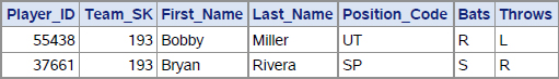
Below is a visual sample for a few players from the file (picked to both satisfy and fail the requirements above). In terms of our subsetting process described above, this file is going to play the role of data collection A.
Output 6.1 Bizarro.Player_candidates Sample

The information about the results at bat for all games in the season is stored in file Dw.AtBats, which does not include the player candidates who have not batted. In our subsetting scheme, it is going to play the role of data collection B. Here is a sample from it for the players listed in Output 6.1:
Output 6.2 Dw.AtBats Sample

Note that this sample does not contain the player with Player_ID=52320 because he is not in the file (meaning that he has not been at bat). Also, though all records with Result="Triple" for these players are included in the sample, only a few records with other results are included, merely for illustrative purposes.
If we used SQL, the following query could be used to achieve the subsetting goal:
Program 6.1 Chapter 6 Simple Subsetting via SQL Subquery.sas
proc sql ;
create table Triples as
select * from bizarro.Player_candidates
where Player_ID in
(select Batter_ID from Dw.AtBats where Result = "Triple")
and Team_SK in (193) ;
quit ;
To get the same result using a hash table, we need three hash table operations:
1. Create to declare, define, and instantiate a hash object.
2. Insert to load its hash table with the key-values of Batter_ID from Dw.AtBats for which Result="Triple".
3. Search to find which Player_ID key-values coming from Bizarro.Player_candidates are in the hash table.
In the snippet below, the DATASET argument tag is used to perform the indirect Insert operation:
Program 6.2 Chapter 6 Simple Subsetting via Hash Table.sas
data Triple ;
if _n_ = 1 then do ; ❶
dcl hash triple ❷
(dataset:'Dw.AtBats(rename=(Batter_ID=Player_ID) ❸
where=(Result="Triple"))') ;
triple.defineKey ("Player_ID") ; ❹
triple.defineData ("Player_ID") ; ❺
triple.defineDone () ;
end ;
set Bizarro.Player_candidates ; ❻
where Team_SK in (193) ;
if triple.check() = 0 ; ❼
* if not triple.check() = 0 ; ❽
run ;
Let us now see how the step above goes about its subsetting business:
❶ Ensure that the Create operation is done only once, on the first iteration of the DATA step implied loop, to prevent the ensuing iterations from dropping the hash table and re-creating it.
❷ Declare hash object Triple and create an instance of it.
❸ At the same time, use the DATASET argument tag to perform the indirect Insert operation by reading data set Dw.AtBats and load the Batter_ID key-values into the table. The data set option RENAME is used to make input variable Batter_ID consistent with the name of hash variable Player_ID defined on the next line. The data set option WHERE is used to select only the batters who have hit a triple. Note that the argument tag MULTIDATA is omitted. Hence, only the first record for each batter who has hit a triple is loaded into the table, and the rest are discarded. It fits the purpose of the task, at the same time reducing the number of hash items (and the hash memory footprint).
❹ Define the key portion of table Triple as a simple numeric key using a single hash variable Player_ID.
❺ For the task at hand, we do not need the data portion since we need only to discover if the key-values coming from Bizarro.Player_candidates are in the table. However, the hash object design requires that we must have the data portion with at least one hash variable in it. The optimal decision is to define it with a single variable to make the least impact on the hash memory footprint. As it turns out from testing on all major platforms, a single numeric variable takes up the least hash memory - in fact, even less than a $1 character variable. In this sense, using numeric variable Player_ID fits the purpose.
❻ Read a record from Bizarro.Player_candidates, bringing the key-value of Player_ID into the PDV.
❼ Perform the Search operation to find if this key-value is in table Triple. The CHECK method doing it is called implicitly because, thanks to the renaming done in ❸, the name of the searched PDV host variable Player_ID is the same as its hash table key counterpart. The CHECK method call is included in the subsetting IF statement, so when it returns a zero code (the key is found), the current PDV content is written as a record to output data set Triple.
❽ Alternatively, the subsetting IF condition can be simply reversed to output the player candidates who have not both batted and hit a triple. Note that it does not carry with it any performance implications like those that sometimes arise when the NOT IN clause is used with SQL.
Running the step above results in the following output for the player candidates from Bizarro.Player_candidates shown in the sample. We get the same output we would get if SQL were used instead:
Output 6.3 Simple Subsetting Results
The subsetting has resulted in the absence of two players from the output:
● Player_ID=52320 – because he has not batted.
● Player_ID=43400 – because, though he has batted, he has not hit a triple.
Note that the MULTIDATA:"Y" argument tag was not specified when the instance of hash table Triple was created. This is because, in the case of pure subsetting, we need to know only the unique values of Player_ID for players who have hit a triple. So, inserting multiple hash items for the same key-value into the table would be extraneous, and all the more so because doing that would only unnecessarily increase the hash memory footprint. Also, it does not matter from which record in Dw.AtBats each unique key-value kept in the table comes, and thus we can leave the choice up to the input process behind the argument tag DATASET (which, out of multiple input keys with the same value, automatically selects the first it encounters). However, as we will see soon later, keeping all hash items sharing the same key-value can be indispensable when the nature of a task calls for it.
6.2.3 Why a Hash Table and Not SQL?
Since we started with an SQL query to make the essence of the subsetting task more evident, a natural question arises: Why not just do it with SQL instead of using a hash table in the DATA step? The answer is two-fold:
● Searching a hash table explicitly may be faster than relying on the internal searching mechanism the SQL optimizer chooses when it decides on the path to execute the query.
● The DATA step language, being procedural, offers certain advantages over the declarative SQL in terms of programming flexibility. Combined with the flexibility of the hash object, it can be used to accomplish, in a natural manner and often in a single data pass, a number of things difficult or impossible to do via a single query (or making the query too convoluted).
From the perspective of the business users, the key advantage of the hash table approach is that multiple subsetting criteria can be easily added. The sport is well known for needing to identify how many times some rare event has happened (e.g., how many players on their first AtBat as professional, who are also pitchers, have hit a home run on the first pitch in the strike zone) in combination with other events..
6.2.4 Subsetting with a Twist: Adding a Simple Count
To illustrate the flexibility point made above, let us add a wrinkle to the task. To wit, suppose that, in addition to selecting the player candidates who have batted and hit a triple, we also want to know how many times each of these players has hit a triple. In order to do it using SQL, we would have to reformulate the query shown above from a subquery to a join and add a GROUP (BY) clause. This is because the SAS rendition of SQL cannot loop through the multiple rows per batter returned by the inner query in case the player has hit more than one triple. For example, the query could be recoded as follows:
Program 6.3 Chapter 6 Subsetting via SQL Join with Simple Count.sas
proc sql ;
create table Triple_Count_SQL as
select p.*, a.Count
from bizarro.Player_candidates p
, (select Batter_ID, count(*) as Count
from Dw.AtBats
where Result = "Triple"
group Batter_ID) a
where a.Batter_ID = p.Player_ID
and p.Team_SK in (193)
;
quit ;
However, to achieve the same result using the hash table Triple in the DATA step explained above, we need not change existing code logic but need only to add the Keynumerate operation to count the hash
items in every same-key item group with a matching Player_ID key (the additions to the DATA step above are shown in boldface):
Program 6.4 Chapter 6 Subsetting via Hash Table with Simple Count.sas
data Triple_Count_Hash ;
if _n_ = 1 then do ;
dcl hash triple (multidata:"Y" ❶
, dataset:'Dw.AtBats(rename=(Batter_ID=Player_ID)
where=(Result="Triple"))'
) ;
triple.defineKey ("Player_ID") ;
* triple.defineData ("Player_ID") ; ❷
triple.defineDone () ;
end ;
set Bizarro.Player_candidates ;
where Team_SK in (193) ;
if triple.check() = 0 ; ❸
do Count = 1 by 1 while (triple.do_over() = 0) ; ❹
end ;
run ;
Here is the summary of the changes:
❶ Adding the MULTIDATA:"Y" argument tag allows duplicate-key items and enables the Keynumerate operation to be performed later.
❷ This call can be omitted because, in its absence, all hash variables defined in the key portion (in this case, single variable Player_ID) are automatically defined in the data portion.
❸ Because of this subsetting IF statement, the DO loop below is executed only if an item group with Player_ID matching the current PDV value of host variable Player_ID is found in the table. Otherwise, program control moves to the top of the step, and the next record from Bizarro.Player_candidates is read.
❹ Perform the Keynumerate operation. The initial DO_OVER method call sets the item list for this key. It always succeeds since the preceding subsetting IF statement ensures that the key-value of host variable Player_ID is in the table. The initial and ensuing DO_OVER calls (which succeed if the player has hit more than one triple) enumerate the item group with the current key-value, thus incrementing the DO loop index variable Count at each iteration. (Note that using the index variable serves the dual purpose of both initializing and incrementing the counter. Thus, it is more compact and convenient than two separate statements to initialize the counter before the loop and then increment it inside it.) The loop terminates when the list set by the initial DO_OVER call has been exhausted because the final DO_OVER call returns a non-zero code, for there are no more items in the item group left to enumerate. After the DO loop is terminated, the implicit OUTPUT statement at the bottom of the step writes a record to output file Triple_Count with the current PDV values, including the aggregate value of Count.
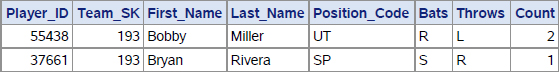
Running the step above will result in adding variable Count compared to the output of simple subsetting:
Output 6.4 Result of Subsetting with Triple Hit Count Added
It is worth noting that by presenting this technique, we have inadvertently waded into the territory outside of the pure Search operation domain. The reason is that the DO_OVER method implicitly performs the Retrieve operation (as part of any Enumerate operation) by extracting the value of data portion hash variable Player_ID into its PDV host variable counterpart. In the example above, it is a mere unavoidable side effect of calling the DO_OVER method, and it is not used for any purpose. However, it becomes the primary effect when it comes to combining data via a hash table. And to reinforce the point made above about the advantages of the procedural nature of the DATA step, metrics could be calculated for teams that have at least 1 player who has, for example, 5 triples.
Both our IT and business users appreciated this wrinkle because they both recognize that virtually every question that is asked that will require a program to be written, will have the inevitable add-on comment, “Great, but can we also do X?”
6.3 Combining Data
In the context of this discussion, combining data means adding non-key data (also termed satellite data) elements from data collection B to data collection A via a common key where the key-values in A and B match. Everything said above about the two principally different subsetting approaches applies equally to combining data. Namely, they are:
1. Sort A and B by their keys and run a sequential match algorithm either explicitly (e.g., using the MERGE statement) or implicitly (e.g., if the SQL optimizer chooses such a path).
2. Insert the key and the satellite information from B in a lookup table. Then read A one record at a time and search the table for the key-value it contains.
The reasons for choosing approach #2 over approach #1 are the same as with the subsetting. Moreover, the coding schemes used for the subsetting and combining tasks are very similar. The principal difference is that when we combine data, we need not merely to establish whether the key-values from A are present in B; but we also need to extract the required satellite information from B for every matching key-value. In other words, instead of performing the pure Search operation against the hash table, we have to perform the Retrieve operation instead. It can be executed in an explicit manner (e.g., by calling the FIND method) or implicitly as part of the Keynumerate or Enumerate All operations depending on the particular situation. A very common use case is adding dimension table variables to a fact table in a star schema data warehouse.
Again, for the benefit of our business users, the need to combine multiple data sources is something that virtually any program that calculates metrics will need to do. There will almost always be data or information that exists in other files that are needed for our analysis. For example, when the manager of a team considers what players to include in the line-up (i.e., as batters) he may want to evaluate how his players have done against the opposing pitcher for today’s game. Given the Bizarro Ball data discussed in Chapter 5, that requires combining data from the Pitches and AtBats data using the appropriate keys to match the data.
6.3.1 Left / Right Joins
In order to see how it works, let us expand the specification for the subsetting task described above. Namely, suppose that for every player record for the Huskies team (Team_SK=193) from file Bizarro.Player_candidates, we want to not merely find from file Dw.AtBats who has batted and hit a triple but also:
● For the players who have batted and scored a triple, add variables Distance and Direction from file Dw.AtBats for all their triple runs. Thus, if a player has scored N triples, that player will have N records in the output.
● For the rest of the players, keep their records from Bizarro.Player_candidates in the output but leave variables Distance and Direction missing to indicate that these players have not both batted and scored a triple.
In terms of set operations, these requirements are equivalent to requesting a left join or right join of Bizarro.Player_candidates with the subset of Dw.AtBats where Result="Triple". They could be satisfied, for example, by running the following SQL query:
Program 6.5 Chapter 6 Left Join via SQL.sas
proc sql ;
create table Triples_leftjoin_SQL as
select p.*
, b.date
, b.Distance
, b.Direction
from bizarro.Player_candidates (where = (Team_SK in (193))) P
left join
Dw.AtBats (where=(Result in ("Triple"))) B
on P.Player_ID = B.Batter_id
;
quit ;
The hash solution below attains the same goal as the SQL query above and is a subtle variation on the program used for data subsetting with a count shown earlier:
Program 6.6 Chapter 6 Left Join via Hash.sas
data Triples_leftjoin_Hash (drop = Count) ;
if _n_ = 1 then do ;
dcl hash triple (multidata:"Y" ❶
, dataset:'Dw.AtBats(rename=(Batter_ID=Player_ID)
where=(Result="Triple"))'
) ;
triple.defineKey ("Player_ID") ; ❷
triple.defineData ("Distance", "Direction") ; ❸
triple.defineDone () ;
if 0 then set Dw.AtBats (keep=Distance Direction) ;
end ;
set Bizarro.Player_candidates ;
where Team_SK in (193) ;
call missing (Distance, Direction) ; ❹
do while (triple.do_over() = 0) ; ❺
Count = sum (Count, 1) ;
output ;
end ;
if not Count then output ; ❻
run ;
The callouts above mark the changes necessary to implement the required left join, as well as some other program lines that warrant explanation:
❶ Adding the MULTIDATA:"Y" argument tag allows duplicate-key items and enables the Keynumerate operation to be performed using the DO_OVER method downstream. In this situation, it is a must because we need to pair each player record on the side of Bizarro.Player_candidates with all of his triple-scoring records in Dw.AtBats. So, each triple-scoring record from Dw.AtBats for a given triple-scorer identified by Batter_ID must have a corresponding hash item in hash table Triple. Storing multiple hash items per key is what enables us to perform one-to-many (or, potentially, many-to-many) matching. Note that before table Triple is loaded via the DATASET argument tag, variable Batter_ID coming from file Dw.AtBats has been renamed as Player_ID for the sake of the simplicity of making the ensuing DO_OVER calls implicit.
❷ We are going to do the matching and retrieval by variable Player_ID; hence, it is defined here as the hash table key.
❸ We need to extract the values of satellite variables (Distance,Direction) from the hash table into the PDV for every Player_ID value from Bizarro.Player_candidates matching the key-values of Player_ID in hash table Triple. Therefore, it is necessary to define them as satellite variables in the data portion of the table. Otherwise, the Keynumerate operation would not be able to retrieve their hash values into the corresponding PDV host variables. The PDV host variables for hash variable Distance and Direction are created by the SET statement at the bottom of the IF-END block. Because of the IF 0 condition it reads no data from Dw.AtBats but lets the compiler place variables (Distance,Direction) in the compiler symbol table and the PDV at compile time. Thus later, at run time, it lets the DEFINEDONE method detect their names and other attributes, validating that the variables defined by the DEFINEDATA method already exist in the PDV.
❹ As we intend to perform an equivalent of a left join, satellite variables (Distance,Direction) in the output must be missing if no match between Player_ID from the current Bizarro.Player_candidates record and Player_ID in the hash table is found. Here we set (Distance,Direction) to missing values beforehand, so that in case the prior record had a match, their retained non-missing values would not persist. Also, testing either variable for a missing value after Keynumerate has done its job can optionally be used to judge whether it found a match or not.
❺ The DO_OVER method is called repeatedly in a DO WHILE loop. If the first call in the loop fails (i.e., returns a non-zero code), it means that no match for the current PDV value of Player_ID exists in table Triple. In such a case, program control exits the loop without executing the OUTPUT statement and incrementing auxiliary variable Count in its body due to the way the WHILE loop operates—and so, nothing is output, and the value of Count remains missing. Otherwise, the first DO_OVER call sets the item list for the matching key-value of Player_ID and retrieves the values of (Distance,Direction) from the first hash item in the item group with this value of Player_ID into their PDV host variables. Then this action repeats for every next item in the same-key item group until the group has no more items to enumerate. Thus, if the item group has N items with this key-value, exactly N records are output.
❻ If a record from Bizarro.Player_candidates has no match in table Triple, it has not been output yet. However, since we are doing a left join, it has to be. Variable Count indicates whether a match has been found or not. If its value is 1 or greater, it has been. Otherwise, its value remains missing, having been automatically reset at the top of the DATA step implied loop. Here we use this indicator to detect and output the records with no match in table Triples and missing values for (Distance,Direction) before the next record from Bizarro.Player_candidates is read.
For our sample players we have already used above, this program produces the following output:
Output 6.5 Left Hash Join of Bizarro.Player_candidates and Dw.AtBats

Players 52320 and 43400 have missing values for (Distance,Direction) for the same reason they are absent from the subsetting output: Player 52320 has not batted, and player 43400, though having batted, has not scored a triple.
Note that the SQL query shown above generates the same data, except that the sequence of rows it outputs is different. This is because the hash solution keeps the relative sequence of rows in the output identical to that in the input files, while SQL has a mind of its own.
At this point our business users have expressed confusion about the difference between a left join and a right join. To our IT users, the answer to the question is both obvious and not terribly relevant. The easiest way to explain the distinction to the business users was to confirm that there really is not much of a difference. Combining the AtBats data with the Pitches data to augment the AtBats data with information from the Pitches data is a left join because we referenced the AtBats data first. If we are combining the AtBats data with the Pitches data to augment the Pitches data with information from the AtBats data, IT folks refer to that as a right join because the Pitches data is listed as the second data set (i.e., is the one on the right side). When they asked if a right join becomes a left join by just reversing the order the data sets are referenced, we replied EXACTLY. Adding that to IT folks, the distinction is important as it can have an impact on the efficiency of the combine operation.
6.3.2 Merging a Join with an Aggregate
Note that in the above example, variable Count played only an auxiliary role, and so it was dropped. However, if it should be desirable to merge its aggregate value with every output record of the player to which it pertains, it can be done in the very same DATA step by executing the DO WHILE loop twice. To achieve that, we need only to (a) keep variable Count and (b) replace the program between the callouts ➍ and ➏, inclusively, with the following construct:
Program 6.7 Chapter 6 Variation on Left Join via Hash with Count.sas
do while (triple.do_over() = 0) ;
Count = sum (Count, 1) ;
end ;
call missing (Distance, Direction) ;
do while (triple.do_over() = 0) ;
output ;
end ;
if not Count then output ;
Essentially, in order to merge the aggregate value of Count back with its player's record, we execute the Keynumerate operation against the same-key item group twice: First, to increment Count, and second, to output the needed records with Count already summed up. If in the current Bizarro.Player_candidates input record the tuple Player_ID has no match in hash table Triple, the output value of Count will remain missing. So, for our sample players, the "merged" output would look like so:
Output 6.6 Left Join Merged with Aggregate Triple Hit Count

An alert reader will notice that a simple count is not the only aggregate that can be merged with the join output. Indeed, nothing above precludes us from merging it with any other aggregate derived from the hash data portion values being retrieved. For example, if we wanted to also augment each output record for the triple-scorers with the values of total and average Distance, we could achieve it by recoding the first DO WHILE loop as follows:
Program 6.8 Chapter 6 Variation on Left Join via Hash with Multiple Aggregates.sas
do while (triple.do_over() = 0) ;
Count = sum (Count, 1) ;
Sum = sum (Sum, Distance) ;
end ;
Average = divide (Sum, Count) ;
As a result, the output would also contain the newly computed aggregates (note that some columns from Bizarro.Player_candidates are omitted to make the display fit the page):
Output 6.7 Left Join Merged with Multiple Aggregates

What makes this on-the-fly aggregation possible is the ability of the Keynumerate operation to visit every hash item in the item group with a given key and implicitly perform the Retrieve operation on each item along the way. Many other examples of using this handy functionality are included elsewhere in the book.
Given that our business users are most interested in calculating metrics which, by definition, require aggregation, they were particularly interested in this functionality.
6.3.3 Inner Joins
At this point, our business users threw up their hands because they did not understand why there was a need for another adjective to describe how to combine data. Once we explained that an inner join simply meant we kept only rows where the keys existed in both data sets, they understood the need for such a requirement and simply decided to let us move on with satisfying the requests of the IT users.
Given that we want to keep only the matching records, we need to perform an equivalent of an inner join. For our sample players above, it would mean that the records with Player_ID in (43400,52320) must not appear in the output. To make it happen, we do not need to add anything to left join code above. Indeed, the line:
* if not Count then output ;
was coded specifically to output non-matching records. So, all we need to do in order to transform the program from the left join into the inner join is to omit this line of code (or comment it out, as shown above). All other properties of the program are retained. Specifically, it preserves its one-to-many joining functionality (or many-to-many in case the "left" file contains records with duplicate keys), as well as the ability to merge aggregate values into the output. Hence, if in the last left join example (with the Distance aggregates added) the conditional OUTPUT statement above were omitted, the output for our sample players would appear as expected from the inner join, i.e., as follows:
Output 6.8 Inner Join with Multiple Aggregates

6.3.4 DO_OVER Versus FIND + FIND_NEXT
The DO_OVER method, used in the examples above to perform the Keynumerate operation, is quite handy and concise. However, it is available only starting with SAS 9.4. If a piece of code is supposed to work under SAS 9.2 and 9.3 as well as 9.4 and higher, there is a remedy already expounded on in the chapter dedicated to the hash table operations. Namely, the construct:
do while (triple.do_over() = 0) ;
<code inside do-while loop>
end ;
can be replaced with the following programming structure (let us call it Style 1):
do _iorc_ = triple.find() BY 0 WHILE (_iorc_ EQ 0) ;
<code inside do-WHILE loop>
_iorc_ = triple.find_next() ;
end ;
The BY 0 construct ensures that the loop can iterate more than once. Also note that using automatic numeric variable _IORC_ instead of RC to capture method codes is a convenient technique since: (a) the variable is freely available in the DATA step, (b) it is not used here for any other purpose (such as capturing SAS index search results), and (c) it is automatically dropped.
Alternatively, a more concise structure can be used that requires no return code variable at all (let us call it Style 2):
if triple.find() = 0 then do UNTIL (triple.find_next() NE 0) ;
<code inside do-UNTIL loop>
end ;
Admittedly, using the combination of the FIND and FIND_NEXT methods is more verbose compared to the DO_OVER method. Yet, it provides the same exact functionality: The aggregation loop with the DO_OVER method shown above would look as follows if DO_OVER were replaced by the FIND + FIND_NEXT combination (using Style 2, for example):
if triple.find() = 0 then do UNTIL (triple.find_next NE 0) ;
Count = sum (Count, 1) ;
TotalDistance = sum (TotalDistance, Distance) ;
end ;
From the standpoint of the hash table operations, the difference between the DO_OVER and FIND+FIND_NEXT is only that FIND performs the direct Retrieve operation, while DO_OVER does it indirectly. Yet, functionally, both techniques do exactly the same. If a key-value (simple or composite) accepted by the methods exists in the table, both set the item list for the given key-value and perform Retrieve on the first item in the list. Otherwise, the loop is terminated without iterating once. The initial FIND is necessary because it is a prerequisite to calling FIND_NEXT - without calling FIND first, the item list for the same-key item group in question will not be set because FIND_NEXT can be called successfully only when the list is already set. Thus, the initial DO_OVER call does exactly what the priming FIND does; and the subsequent FIND_ NEXT calls do exactly what the subsequent DO_OVER calls do.
6.3.5 Unique-Key Joins
Note that all the data-combining examples above were presented with the assumption that the data to be loaded into the hash table for lookup may contain more than one item per key. Accordingly, the argument tag MULTIDATA:"Y" was used to accommodate multiple items per key-value (and thus enable the Keynumerate operation to retrieve the data from each same-key item). It often happens, though, that the keys in the data to be loaded is intrinsically unique; and so they will remain unique in the hash table after it is loaded. The question then arises: Do we have to change anything in the joining code schemes discussed above in order to account for the fact that the keys in the table are now unique?
The answer is "No", for the Keynumerate operation as coded above handles this case automatically. For a given key-value, the DO loop performing the operation executes its body exactly as many times as there are items for this key-value in the table. If the keys in the table are unique, the same-key item group has only one item, and so the body of the loop is executed only once - just as needed. Let us take another look at both variants of the DO loop which executes the operation:
do while (triple.do_over() = 0) ;
Count = sum (Count, 1) ;
output ;
end ;
and
do _iorc_ = triple.find() by 0 while (_iorc_ = 0) ;
Count = sum (Count, 1) ;
output ;
_iorc_ = triple.find_next() ;
end ;
Let us see what happens in two possible cases: (1) the current key-values in the PDV have no match in the table and (2) they do.
1. The current PDV value of Player_ID has no match in the hash table:
◦ In the variant with DO_OVER, the very first DO_OVER call returns a non-zero code making the WHILE condition false. Hence, program control exits the loop immediately without executing the statements in its body even once. The value of Count remains missing, and no records are output.
◦ In the variant with the FIND+FIND_NEXT combination, exactly the same happens, except that it is the failure of the FIND method that triggers the immediate termination of the loop.
2. The current PDV value of Player_ID does have a match in the hash table:
◦ In the DO_OVER variant, the first DO_OVER call is successful, and the body of the loop is executed, adding 1 to Count and outputting the record. Since the table has no more items for the current key, the next call to DO_OVER at the top of the loop fails and program control exits the loop. Hence, for the only item in the same-key item group, the body of the loop is executed only once.
◦ In the variant with FIND+FIND_NEXT, the same happens, except that it is the successful FIND call that lets the loop iterate for the first time and process the only available item, and it is the non-zero code returned by the ensuing FIND_NEXT that prevents the loop from iterating further.
Thus, the Keynumerate joining scheme works perfectly fine regardless of whether the hash keys have duplicates or not. The only reason to deviate from it is to utilize the fact that the keys are unique to make the program simpler and terser by replacing the Keynumerate operation with the Retrieve operation. For example, in the case of the left join, we can omit the MULTIDATA argument tag altogether and replace the block of code:
call missing (Distance, Direction) ;
do while (triple.do_over() = 0) ;
Count = sum (Count, 1) ;
output ;
end ;
if not Count then output ;
with mere:
call missing (Distance, Direction) ;
_iorc_ = triple.find() ;
The assigned call to FIND is used to prevent errors appearing in the SAS log in case the value of Player_ID present in the PDV at the time of the FIND call has no match in the hash table. The OUTPUT statement is omitted because at the bottom of the DATA step it is implied. Output occurs regardless of whether FIND succeeds or fails. If it fails (i.e., there is no match), the record is output with the (Distance,Direction) pair having missing values, just as required by in a left join; otherwise, they will have the values retrieved from the hash table for the current PDV key-values.
If we are to perform the inner join rather than left join, this is further reduced to:
call missing (Distance, Direction) ;
if triple.find() = 0 ;
In this case, the subsetting IF statement outputs the record only if we have a match.
For a complete example of joining with a file where the key is unique, suppose that we want to know which player candidates in file Bizarro.Player_candidates from team Huskies (Team_SK=193) have actually pitched and in how many unique games each. In order to demonstrate this we need to use a data set created in Chapter 7. The data set Dw.Players_positions_played is a subset of bizarro.Player_candidates and includes a numeric variable Pitcher which is how many games the player has appeared as a pitcher.
Below, is a glimpse of this data set for our four sample players (only the variables in question are shown). Variable Pitcher indicates in how many unique games the player has pitched; if he has not pitched, its value is missing. The key-values of Player_ID are unique throughout the file.
Output 6.9 Sample from Data Set Dw.Players_positions_played

Let us also recall that for our sample of player candidates from team Huskies (Team_SK=193), the corresponding records look as follows:
Output 6.10 Sample from Data Set Bizarro.Player_candidates (Team Huskies)

Therefore, we can code:
Program 6.9 Chapter 6 Unique-Key Left or Inner Join via Hash.sas
data Pitched ;
if _n_ = 1 then do ;
if 0 then set dw.Players_positions_played (keep=Player_ID Pitcher) ;
dcl hash pitch (dataset: "dw.Players_positions_played (where=(Pitcher))") ; ❶
pitch.defineKey ("Player_ID") ;
pitch.defineData ("Pitcher") ;
pitch.defineDone () ;
end ;
set bizarro.Player_candidates ;
where Team_SK in (193) ;
call missing (Pitcher) ; ❷
_iorc_ = pitch.find() ; /*Left join*/ ❸
* if _iorc_ = 0 ; /*Inner join*/ ❹
* if pitch.find() = 0 ; /*Inner join*/ ❺
run ;
This example warrants a few notes:
❶ The MULTIDATA:"Y" argument tag is omitted since there are no duplicate key-values in the input. The SET statement at the top of the IF-DO-END block is used to create the PDV host variables for hash variables Player_ID and Pitcher. Doing parameter type matching in this manner ensures that the host and the hash variables inherit their attributes from the like-named variables in file Dw.Players_positions_played. Also, doing it before the MISSING routine is called downstream guarantees that it will populate variable Pitcher with a missing value of the correct data type.
Note that (Pitcher) is used in the WHERE clause as a Boolean expression. It evaluates true if the value of Pitcher is neither missing nor zero; otherwise, it evaluates false.
❷ Ensure that in the case of left join, the output values of the added satellite variables (here, just variable Pitcher) have missing values if the current PDV value of Player_ID has no match in hash table Pitch.
❸ The FIND method is called to perform the Retrieve operation. It is called assigned to prevent log errors if there is no match for the current PDV value of Player_ID in the table. If the next line is omitted (or remains commented as shown), the operation results in the left join since the output is created for every record from Bizarro.Player_candidates regardless of whether its value of Player_ID has a match in table Pitch or not.
❹ If this line of code is uncommented, the records for which there is no match are not written to the output. In other words, it results in the inner join.
❺ If the inner join is required, both lines ❸ and ❹ can be replaced with this single line. In this case, if the FIND method fails, it does not generate errors in the log because it is called as part of a conditional statement.
In the case of a left join, this is the output we get from the program for our sample:
Output 6.11 Results of Unique-Key Left Join

If the inner (equi-) join is opted for instead, the output will have only the rows with the non-missing values for Pitcher:
Output 6.12 Results of Unique-Key Inner (Equi-) Join

6.4 Splitting Data
At times, we need to accomplish a task opposite to combining data, i.e., to split a data set in a number of data sets in a specific manner. For instance, suppose that we have a data set with N distinct key-values of some ID variable (or a combination of variables) and need to split it into N separate data sets whose names are identified by the corresponding key-values.
For the benefit of our business users, we decided to point out that just one of the benefits of splitting data is that it can make the calculation of certain metrics easier. We provided several examples of such use cases that we felt they could relate to: treating starting pitchers differently than relievers in terms of what pitching related metrics are of interest; treating AtBats for pinch hitters differently from starters. This point prompted the IT users to consider the possibility of different kinds of metrics to include in the project once the Proof of Concept effort is completed.
Returning to the focus of satisfying the curiosity of the IT users, as a simple example, let us look at a subset of file Bizarro.Teams where only a few teams from each league are shown:
Output 6.13 Data Set Bizarro.Teams - Sorted Sample

As outlined above, the task is to split the file into two separate files named League_1 and League_2 and containing the records with League_SK=1 and League_SK=2, correspondingly. It is surely reasonable to ask why such a thing may be needed. Indeed, whatever has to be done against the separate files can be done against the original file using, for example, BY processing logic. The answer is that it is often demanded by business end users. For example, they may want to create a separate sheet in a workbook for each key-value present in the original file.
The traditional approach to this task seems to be very simple:
Program 6.10 Chapter 6 Splitting Data - Hard Coded.sas
data League_1 League_2 ;
set Bizarro.Teams ;
select (League_SK) ;
when (1) output League_1 ;
when (2) output League_2 ;
otherwise ;
end ;
run ;
The advantages of this method are: (a) apparent simplicity, and (b) no need to have the file sorted or grouped by the key variable(s), in this case by League_SK. However, there are a few reefs lurking beneath this quiet surface:
● We have to discover all the distinct ID values beforehand.
● The output data set names in the DATA and SELECT statement have to be typed in - in other words, hard-coded - with that knowledge in mind.
● Hard-coding can be avoided by pre-processing the file to find out what the distinct ID values are and use the result to construct the DATA and SELECT statements programmatically by using a macro or other means of generating code. It means, however, that we need to make two passes through the input file.
● This is true even if the input file is pre-sorted by the ID variable. Though in such a case we can use BY processing to write the records from each BY group to its own file named after the respective key-values, these files must be listed in the DATA statement - they cannot be created at run time on the fly.
With the hash object, however, it is different: It has its own I/O facilities independent from those of the DATA step proper; and thus it can create, name, write, and close output data sets at run time. Let us see what hash table operations we need to make it happen and how.
6.4.1 Hash Data Split - Sorted Input
When the input file to be split is sorted or grouped by the ID variable (which is the case with file Bizarro.Teams sorted by variable League_SK), the operational plan is simple:
On the first iteration of the DATA step implied loop (first DATA step execution), use the Create operation to create a hash table instance.
1. Process the input file one BY group at a time.
2. For each record in the current BY group, use the Insert operation to add its PDV values to the hash table as a new item.
3. After the last record in the current BY group has been read, use the Output operation to: (a) create a new output file with the current value of the ID variable (converted to a character string if it is numeric) as part of the file's name, (b) open it, (c) write the data portion content from the hash table to it, and (d) close it. Then use the Clear operation to purge all items from the hash table without deleting the table itself.
4. Read the next BY group, i.e., go to #1.
The most convenient programming structure to process BY groups one at a time is the DoW loop, as it naturally isolates the programming actions taken before, during, and after each BY group. Thus, we can code:
Program 6.11 Chapter 6 Splitting Sorted Data via Hash.sas
data _null_ ; ❶
if _n_ = 1 then do ; ❷
dcl hash h (multidata:"Y") ; ❸
h.defineKey ("_n_") ; ❹
h.defineData ("League_SK", "Team_SK", "Team_Name") ; ❺
h.defineDone () ;
end ;
do until (last.League_SK) ; ❻
set bizarro.Teams ;
by League_SK ;
h.add() ; ❼
end ;
h.output (dataset: catx ("_", "work.League", League_SK)) ; ❽
h.clear() ; ❾
run ;
This program is quite instructive in spite of its brevity; so let us take a closer look:
❶ Since all output in the step will be handled by the hash object, we do not need to list any output data set names in the DATA statement, which is why it is left with the _NULL_ specification.
❷ This IF-DO-END block contains statements and method calls performing the Create operation. Note that this is done only at the first execution of the DATA step since we intend to keep table H created here across all iterations of the DATA step implied loop- or, to put it another way, across all BY groups we are going to process.
❸ Coding MULTIDATA:"Y" allows multiple items with the same key-value in the hash table. As we will see later, it is not mandatory. However, it comes in handy because we can have the same key-value for every item inserted into the table from a given BY group. As we already know, for the hash items in an item group sharing the same key, their logical order in the table is the same in which they are received. Thus, when the data loaded from each BY group is written from the table to its respective output file, the relative order of the records in the input will be automatically replicated in the output without the need to program for it.
❹ The program plan does not require the table to be keyed - it merely intends to use the hash table as a queue. However, since no hash table can exist without a key, we need to pick one. _N_ is a good choice because: (a) it is freely available, shortest possible, and automatically dropped; and (b) owing to the DoW loop, the value of _N_, after it is incremented at the top of the step in each of its executions, persists for the duration of each corresponding BY group. Thus, it persists for the duration of the first BY group _N_=1, for the second - _N_=2, and so on. So, using _N_ in this manner serves to implement the above idea of having all items related to a given BY group keyed by the same value.
Note that as an equally good alternative, automatic variable _IORC_ could be used instead of _N_, in which case the key-value for any BY group would be the same, namely, _IORC_=0.
❺ Include the variables to be written to the output "split" files in the data portion of the table. The like-named PDV host variables for them will be created when the compiler processes the ensuing SET statement referencing data set Bizarro.Teams whose descriptor contains them. Thus, no extra code is needed for the parameter type matching.
❻ Launch the DoW loop (comprising the lines of code between the DO and END statements, inclusively). It will iterate through every record in the current BY group and terminate after the last record in the group has been read. On this last record, the SET statement in the presence of the BY statement sets last.League_SK=0, and so program control exits the loop at its bottom because of the UNTIL condition.
❼ Call the ADD method to perform the Insert operation. Because of MULTIDATA:"Y", no unduplication occurs, so every input record will have its item counterpart in table H. Thus, inserting an item with a duplicate key-value cannot cause the ADD call to fail. Also, since the key-value of hash variable _N_ stays the same for the entire current BY group, the items inserted into the table end up there in the order they are received, as explained in ➌.
❽ At this point in the control flow, the data from the BY group processed in the current execution of the DATA step has been loaded into table H. Now the Output operation is performed by calling the OUTPUT method. The name of the file to which the data should be written is constructed on the fly by the expression supplied to the argument tag DATASET. The expression uses the CATX function to incorporate the current value of the ID variable (i.e., League_SK) in the name of the output data set. If a file with this name exists, it is deleted and re-created (i.e., over-written); if not, a new file is created. Then the method call causes it to be opened; after the data from all hash items currently in the table has been written to it, it is closed.
Note that this file is locked only during the time the Output operation is being performed (i.e., while records are still being written to it). After the method call has closed, the file it is no longer locked and can be used (for example, opened, browsed, edited, etc.), even though the DATA step still keeps running. This is in sharp contrast with the situation where the name of an output file is listed in the DATA statement and written into by the OUTPUT statement (explicit or implicit) because in this case, the file is not closed until the DATA step has finished running.
❾ Perform the Clear operation by calling the CLEAR method. Reason: The next iteration of the DATA step implied loop is going to process the next BY group. Since all our work with the current BY group has now been finished and its content written out to the corresponding output file, we no longer need the data from the current BY group in the table. Instead, we need to purge the items currently in the table without deleting the table, so that we will have the table empty and ready to receive the data from the next BY group.
Running the DATA step shown above generates the following notes in the SAS log:
NOTE: The data set WORK.LEAGUE_1 has 16 observations and 3 variables.
NOTE: The data set WORK.LEAGUE_2 has 16 observations and 3 variables.
NOTE: There were 32 observations read from the data set BIZARRO.TEAMS.
And the output content for the two files League_1 and League_2 looks as follows (only the first 2 records for League_SK=1 and the first 3 records for League_SK=2 are displayed):
Output 6.14 Result of Splitting File Bizarro.Teams for League_SK=1

Output 6.15 Result of Splitting File Bizarro.Teams for League_SK=2

Note that the relative sequence of records coming from Bizarro.Teams has been maintained intact.
Let us now consider a couple of code variations. First, we have mentioned earlier that coding MULTIDATA:"Y" is not mandatory to achieve the goal. (In fact, if you are running SAS 9.1 - which, against all odds, still may happen - the MULTIDATA argument tag is not even available.) If it is not used, it must be ensured that for each record read from a given BY group, a corresponding item is inserted into table H. But since without MULTIDATA:"Y" duplicate-key items are not allowed, we must guarantee that for each item we attempt to insert into the table, the key-value is different. This is easy to achieve by recoding the program as follows (the changes are shown in bold):
Program 6.12 Chapter 6 Splitting Sorted Data via Hash with Unique Key.sas
data _null_ ;
if _n_ = 1 then do ;
dcl hash h (/*multidata:"Y"*/ ordered:"A") ; ❶
h.defineKey ("unique_key") ;
h.defineData ("League_SK", "Team_SK", "Team_Name") ;
h.defineDone () ;
end ;
do unique_key = 1 by 1 until (last.League_SK) ; ❷
set bizarro.Teams ;
by League_SK ;
h.add() ;
end ;
h.output (dataset: catx ("_", "work.League", League_SK)) ;
h.clear() ;
run ;
❶ The argument tag ORDERED:"A" guarantees that the items which are now uniquely keyed are inserted into table H in the order they are received from the input. In fact, coding this way programmatically enforces that the relative input record sequence is replicated in the output irrespective of the internal hash table order maintained by default in presence of the argument tag MULTIDATA:"Y".
❷ Incrementing unique_key up by 1 for every new record in a given BY group ensures that every item in the table is keyed by its own unique key-value.
There is another interesting variation on the same theme related to the Clear operation. If you are perchance still running SAS 9.0 or 9.1, the CLEAR method is not available. One alternative is to use the combination of the Delete (table) and Create operations instead to delete the entire instance of H (and its content with it) after each BY group has been processed and re-create it anew before the next BY group. Or, in the SAS language:
Program 6.13 Chapter 6 Splitting Sorted Data via Hash with DELETE Method.sas
data _null_ ;
* if _n_ = 1 then do ;
/*Create operation code block*/ ❶
dcl hash h (ordered:"A") ;
h.defineKey ("unique_key") ;
h.defineData ("League_SK", "Team_SK", "Team_Name") ;
h.defineDone () ;
* end ;
do unique_key = 1 by 1 until (last.League_SK) ;
set bizarro.Teams ;
by League_SK ;
h.add() ;
end ;
h.output (dataset: catx ("_", "work.League", League_SK)) ;
* h.clear() ;
/*Delete the instance of object H*/
h.delete() ; ❷
❸
run ;
Here is how it works:
❶ Now that the Create operation code block is executed unconditionally, the operation is performed every time program control passes through the block- i.e., for each new value of _N_, thus causing the instance of object H to be created before each respective BY group is processed.
❷ After the BY group is processed and the respective "split" file is written out, the DELETE method call erases the instance of H. Note that this call is optional (see ❸ below) and can be omitted.
❸ Program control from this point loops back to ❶ - the top of the DATA step for its next execution. The instance of H just erased at the bottom of the step is re-created.
This variant will work with any SAS version starting with 9.0. Be mindful, though, that the processing cost of doing so is much higher (by an order of magnitude or so) than merely clearing the content of the persisting table. If you have but a few BY groups in the input file, you are not likely to notice any run-time difference. Yet, if they are very numerous, it may render the program annoyingly slow. So, with SAS 9.2 or higher it is much more sensible to let the hash object persist and use the Clear operation to purge it before every BY group.
6.4.2 Hash Data Split - Unsorted Input
If the input file is not sorted or grouped by the ID variable, using BY processing as demonstrated above is not an option. Suppose that input file Bizarro.Teams was not intrinsically sorted by League_SK and our few sample records looked as follows:
Output 6.16 Data Set Bizarro.Teams - Unsorted Sample

It raises the question: Is it still possible to do the data split in a single pass through the input file? Actually, the answer is "Yes", and it is based on the ability of the SAS hash object to store data pointing to hash object instances. Let us see what a logical plan for such a program could be:
1. Read the file.
2. Every time a new value of League_SK is encountered, fully define (i.e., with keys and data) and create a new instance of the hash object H for this value of League_SK. Store the value of League_SK, along with some variable pointing to (or identifying) the related instance, in some suitable data structure, so that later on it can be accessed to identify this instance using League_SK as a key.
3. For every record, identify the hash instance related to the current PDV value of League_SK. Then perform the Insert operation to add an item with the data from this record to the hash table associated with this value of League_SK.
4. After the file has been read, go through the stored instances of H one at a time. For each, perform the Output operation to output the "split" file named after the value of League_SK identifying its own instance of H.
There is only one little problem with this plan: In order to "go through the stored instances of H", we need to save the pointers identifying these separate instances as data in some enumerable data structure keyed by League_SK. A regular SAS array is an enumerable data structure. However, it is ill suited for the purpose since it can house only scalar data, while a pointer to an object instance represents non-scalar data (of type hash object). However, a hash table (which, if you will recall, is also termed an associative array) is a perfect container for data of this type and so, just as any hash table, can be keyed by League_SK.
We are wading into the territory of what is termed Hash of Hashes (HoH) treated in detail in the corresponding chapters later in the book. Therefore, here we will limit the discussion to a working program annotated only to show how it corresponds to the plan devised above:
Program 6.14 Chapter 6 Splitting Unsorted Data via Hash of Hashes.sas
data _null_ ;
if _n_ = 1 then do ;
dcl hash h ; ❶
dcl hash hoh() ; ❷
hoh.defineKey ("League_SK") ;
hoh.defineData ("h", "League_SK") ;
hoh.defineDone () ;
end ;
set bizarro.Teams end = lr ; ❸
if hoh.find() ne 0 then do ; ❹
h = _new_ hash (multidata:"Y") ; ❺
h.defineKey ("_iorc_") ; ❻
h.defineData ("League_SK", "Team_SK", "Team_Name") ;
h.defineDone () ;
hoh.add() ; ❼
end ;
h.add() ; ❽
if lr ;
dcl hiter ihoh ("hoh") ; ❾
do while (ihoh.next() = 0) ;
h.output (dataset: catx ("_", "work.League", League_SK)) ; ➓
end ;
run ;
❶ Declare a hash object named H. This has the effect of creating a non-scalar (of type hash object) PDV variable H. At any point in the program, its value identifies the hash object instance associated with it.
❷ This statement and the following three method calls perform the Create operation to create hash table HoH. Its key is hash variable League_SK; and the data portion includes hash variables H and scalar variable League_SK. The host variable for H is created by the statement ➊; and the host variable for League_SK - by the SET statement downstream.
❸ Read the next record from the input file.
❹ The FIND method searches table HoH for the current PDV value of League_SK. If it is there, it retrieves the related value of hash variable H (i.e., the pointer to the related instance of H) into the host variable H.
❺ Otherwise, a new distinct value for PDV host variable H is created by the _NEW_ operator. The rest of the calls in this IF-DO-END block perform the Create operation to fully define and create a new instance of H associated with this new value.
❻ Note that all instances of hash object H are defined with key variable _IORC_ which will have the same default value _IORC_=0 for all items in every instance of H throughout the program. Thus, _IORC_ plays the role of a convenient key portion placeholder in the situation where, because of MULTIDATA:"Y", the key portion has no practical function for the instances of H used as simple FIFO (First In - First Out) queues.
❼ The ADD method is called to perform the Insert operation, adding the current PDV value of League_SK and the related value of H to table HoH as a new item with the new distinct key-value of League_SK. Since ADD is called only if this value is not already in the table, the method is guaranteed to succeed and thus can be called unassigned.
❽ Perform the Insert operation to add an item to the instance of H linked to the current PDV value of League_SK. The instance is identified by the current value of PDV host variable H. At the time of this ADD call, this variable has been valued in one of two ways:
(a) If the current PDV value of League_SK is new, i.e., it was not in table HoH when FIND was called at ❹, then H also has a new value assigned by the _NEW_ operator and identifying the new instance of H the operator has just created.
(b) Otherwise, it is the hash value of H just retrieved from HoH by the FIND call using the PDV value of League_SK as its key-value.
Either way, now the value of H identifies the specific instance of H linked to the current PDV value of League_SK, and thus this is the instance into which the H.ADD() call inserts a new item with the values of League_SK, Team_SK, and Team_Name from the current record.
❾ Now that all input records have been processed (which occurs when LR=1 is set), we need to scan through the instances of H uniquely related to the distinct values of League_SK and, for each, output a "split" file with the name identified by its own value of League_SK and the data content of the corresponding hash table instance. Therefore, we need to perform the Enumerate All operation against table HoH. Here, it is made possible by creating hash iterator iHoH explicitly linked to table HoH.
The enumeration itself is performed by the DO WHILE loop repeatedly calling the hash iterator method NEXT until it returns a non-zero code when no more items are left to enumerate. In each iteration of the loop, NEXT retrieves the interrelated hash values of H and League_SK from the data portion of the next item of table HoH into their respective PDV host variables. Thus, for each enumerated item, when the PDV host variable H is overwritten with the value of its hash counterpart, its value now points to the specific instance of H on which to operate; and it is correctly paired in the PDV with the value of League_SK to which it is related.
Note that hash variable League_SK is included in the data portion of HoH (in addition to being included in the key portion) on purpose. Otherwise, the NEXT method would not be able to retrieve its values from the table into the PDV host variable League_SK, as only the data portion hash variables are retrievable.
❿ The OUTPUT method reads the data from the hash instance identified by the PDV value of H and writes its data portion content into the "split" file identified by the PDV value of League_SK to which the instance is linked.
This program generates the same output and log notes as the prior example where BY processing is used. It is evidently more dynamic in the sense that it does not require the input file being split to be sorted or grouped by the ID variable. However, it has two shortcomings. First, it needs more memory, as eventually all the input data ends up loaded into memory before the "split" files are output. Second, being based on the "hash of hashes" concept, it is admittedly more complex. However, we feel that it can serve as a good propaedeutic teaser for the chapters later in the book where the "hash of hashes" techniques are explored in much more detail and put to better use. Though you will see the notions outlined above reiterated, perhaps at different angles, it may be a good thing: As the Latin proverb says, "Repetitio est mater studiorum".
6.5 Ordering and Grouping Data
The ORDER operation packaged with the hash object via the argument tag ORDERED is what makes it a handy data-ordering tool and has a number of useful applications. In addition, the intrinsic hash object structure working behind the scenes when the argument tag MULTIDATA:"Y" is specified makes it possible to group data without sorting it, thus avoiding the extra expense of the latter.
At this point our business users did not need an explanation of why this was an important capability. Grouping the data to calculate metrics for each batter (just one example) made perfect sense to them- as did the idea of ordering the result sets by the batter’s team and/or name.
Let us say from the outset that the data sorting capability of the hash object cannot and does not replace the functionality, efficiency, and capacity of the procedures (such as SORT and SQL) specifically designed for the purpose, particularly for sorting massive data. Moreover, the hash object has no provision (at least as of SAS 9.4) for sorting in both ascending and descending order by different key components within a composite key: All that the hash object can do is sort either descending or ascending by the entire key as a whole.
However, there are many use cases where the ability of the hash object to sort or group comes in very handy. For example (the list does not pretend to be exhaustive):
● The logic of a DATA step program requires that the data in a hash table be sorted by its key. In this case, using the ORDERED argument tag makes it unnecessary to pre-sort the data before loading it into the table.
● After the hash data has been processed (e.g., after a number of table updates or computing aggregates), it is written out to a data set required to be in a sorted order. For example, the latter may be needed just to make the result more convenient to view or if the output needs to be reprocessed using the BY statement. In these cases, having the output already ordered eliminates an extra sorting step.
● It is desirable to sort a DATA step structure different from a hash table at run time but the inherent DATA step functionality to do so is either absent or limited. Sorting a set of parallel arrays might be a good example.
● BY group post-processing. The idea is to load data from every input BY group into a number of hash tables, each ordered differently, to obtain a number of group metrics by enumerating each table based on its own order. Then the tables can be cleared to process the next group identically. As a simple example, suppose that we need to compute percentiles for N different variables for each BY group. A head-on method would require re-sorting the entire input and rereading it N times, which can be prohibitively costly. Yet, using the approach outlined above, the job can be done in a single pass using N hash tables - at a mere fraction of the cost.
Since we have discussed the ins and outs of the Order operation at the detailed level earlier, we will limit this section to a few sparsely annotated practical examples. You will also find numerous examples of using the operation matter-of-factly elsewhere in the book, particularly in the programs generating the sample data.
6.5.1 Reordering Split Outputs
First, let us revisit the task of splitting sorted data discussed in the preceding section. There, we already had a hint of using the argument tag ORDERED to impose the replication of the input record order on the "split" output files in the absence of MULTIDATA:"Y". Now suppose that instead, we want the "split" files related to each League_SK to be ordered by Team_SK. Surely, we can do it in a later step by re-sorting them. However, there is a better way:
Program 6.15 Chapter 6 Reordering Split Outputs.sas
data _null_ ;
if _n_ = 1 then do ;
dcl hash h (multidata:"Y", ordered:"A") ; ❶
* h.defineKey ("_n_") ;
h.defineKey ("Team_SK") ; ❷
h.defineData ("League_SK", "Team_SK", "Team_Name") ;
h.defineDone () ;
end ;
do until (last.League_SK) ;
set bizarro.Teams ;
by League_SK ;
h.add() ;
end ;
h.output (dataset: catx ("_", "work.League", League_SK)) ; ❸
h.clear() ;
run ;
Now the output for our five sample teams will appear sorted by Team_SK:
Output 6.17 Result of Splitting File Bizarro.Teams for League_SK=1 Sorted by Team_SK

Output 6.18 Result of Splitting File Bizarro.Teams for League_SK=2 Sorted by Team_SK

All we had to do in order to achieve it was to ❶ add the argument tag ORDERED:"A" and ❷ replace the dummy key _N_ with Team_SK, leaving everything else intact. If we rather wanted the output to be sorted by Team_Name, we would key the hash table by this variable instead.
Let us reiterate that though the output "split" files are thus intrinsically sorted by Team_SK, the OUTPUT method does not set the SORTEDBY= data set option accordingly and does not add it to the metadata. To save processing time in case an extraneous sort step is added downstream, we can add it by changing line ❸ above as follows:
h.output(dataset:catx("_", "work.League",League_SK,"(sortedby=Team_SK)")) ;
In this case, if an attempt were made to use the SORT procedure to order League_1 or League_2 by Team_SK, it would detect that the data was already in order and skip sorting, only printing a note to that effect in the SAS log:
NOTE: Input data set is already sorted, no sorting done.
6.5.2 Intrinsic Data Grouping
To recap our earlier discussion of the key order of the items in a hash table, they are always logically stored as intrinsically grouped. It means that all items with the same key-values are always stored adjacent to each other, thus forming the same-key item groups. Inside each group, the relative sequence of the items exactly replicates the sequence in which they have been inserted into the table. By default, the groups themselves are, in general, not in key order relative to each other. Now, if a specific order is imposed by using the properly valued argument tag ORDERED, the groups will be also in order relative to each other with respect to the key-value of each group. The matrix below visually encapsulates these differences using a sequence of 7 key-values as an example:
Figure 6.1 Ungrouped Unsorted vs Grouped Unsorted vs Grouped Sorted

To see what occurs using real data, let us extract a small sample from data set Bizarro.AtBats where:
● The team is Huskies; Team_SK=193.
● The batter is a starting pitcher; Position_code="SP".
● The batter has hit a single or double; Result="Single" or Result="Double".
● The games are home games; Top_Bot="B" (the home team bats at the bottom of the inning).
● The games have been played in 2017 between March 20 and April 9.
Program 6.16 Chapter 6 Sample from AtBats.sas
data Sample (keep = Batter_ID Result Sequence) ;
set bizarro.AtBats ;
where Team_SK = 193 and Position_code = "SP" and Top_Bot = "B"
and date between "20mar2017"d and "09apr2017"d
and Result in ("Single", "Double") ;
Sequence + 1 ;
run ;
We created variable Sequence as a unique ID for each row indicating the sequence of the observations in Sample. This is the order in which the observations in Sample will be loaded into a hash table. The content of the sample file looks as follows:
Output 6.19 Sample from Bizarro.AtBats with a Sequence Variable


Now let us load the file into a hash table without imposing a specific order on it and then output the content of the table to file Grouped:
Program 6.17 Chapter 6 Intrinsic Hash Table Grouping.sas
data _null_ ;
dcl hash h (multidata:"Y") ;
h.defineKey ("Batter_ID") ;
h.defineData ("Batter_id", "Result", "Sequence") ;
h.defineDone () ;
do until (lr) ;
set Sample end = lr ;
h.add() ;
end ;
h.output (dataset: "Grouped") ;
stop ;
run ;
Note that no ORDERED argument tag is specified; hence, the table is ordered by internal default. The content of file Grouped written by the OUTPUT method call looks as follows:
Output 6.20 Grouped Output from an Unordered Hash Table

As we can see, the file is now grouped by Batter_ID. (Note also that the relative input sequence within each same-key group is maintained.) It means that although it is not sorted, if we now needed to use the BY statement to process it one BY group at a time, it would be just as good as if it were sorted, for we could code:
set Grouped ;
by Batter_ID NOTSORTED ;
without any fear that the result could be inaccurate - as it would be if the file were neither sorted nor grouped.
6.6 Summary
The goal of this chapter was to get the buy-in of the IT users. They appreciated that of many data processing problems that can be successfully addressed using the hash object, the tasks discussed in this chapter represent a small sample of rather simple scenarios. Their choice is mainly dictated by the need to illustrate the principle of applying a specific hash table operation to perform a specific programming action according to the nature of the task. In the ensuing chapters, we will see how other, more complex, tasks that address capabilities of particular interest to the business users can be tackled with the aid of the hash object. However, the hash operations approach delineated in this chapter will remain the same.