
Chapter 10: The Hash Object as a Dynamic Data Structure
10.2.1 Basic Stable Unduplication
10.2.2 Selective Unduplication
10.3 Testing Data for Grouping
10.3.2 Using a Hash Table to Check for Grouping
10.4 Hash Tables as Other Data Structures
10.4.4 Using a Hash Stack to Find Consecutive Events
10.5.1 Using a Hash Table to Sort Arrays
10.1 Introduction
There exist a great variety of practical data-processing scenarios where programming actions must be taken depending on whether or not a current value in the program has already been encountered during its execution. In order to do it, some kind of data structure must be in place where each distinct current value can be stored for later inquiry and then looked up downstream as quickly as possible.
SAS provides a number of such structures, such as the arrays, string-searching functions, the LAG function, etc. In the simplest case, even a single temporary variable may fill the role. However, in terms of structures that are both convenient and fast, no other structure rivals the hash table because of its ability to store, look up, retrieve, and update data in place in O(1) time. Moreover, since the hash table can grow and shrink dynamically at run time, we need not know a priori how many items will have to be added to it.
In this book, we have already seen many cases of exploiting this capability without stressing it. In this chapter, examples will be given with the emphasis on this feature of paramount importance, as well as the hash operations needed to perform related tasks.
For the benefit of our business users, we explained that the rationale here is simply that the hash object allows us to answer a number of questions more quickly. For example, how many times have both teams scored more than some number of runs in the first inning; how many times have all nine batters gotten a hit. And the question is not only how often has it happened: The information about each occurrence also needs to be presented.
For the benefit of our IT users, this chapter expands upon the data tasks discussion in Chapter 6.
10.2 Stable Unduplication
To unduplicate a file means to select, from all records with the same key-value, just one and discard the rest. Stable means that in the output file to which the selected records are written, the original relative sequence of the input records is preserved. Which record with a given key-value should be selected depends on the nature of the inquiry. Here are just some possible variations:
1. The records have been entered into the file chronologically, and it may be of interest to know which record with the given key-value occurs first or last.
2. A file (e.g., extracted from a data warehouse) may contain multiple records with the same key-value, each marked by the date of its insertion, and for each key-value, we need to keep the record with the latest date since it has the most recent information.
3. Whole records in a file may have been duplicated for one or another reason, and it may be necessary to discard the duplicates in order to cleanse the data. In this case, it does not matter which same-key record to pick.
In scenarios #1 and #2, our business use case is to find all of the times some event has happened subject to some constraints.
10.2.1 Basic Stable Unduplication
Let us look, as an example, at our sample data set Dw.AtBats. Its records represent events entered into the file chronologically – i.e., the event reflected by any record occurred later than the event reflected by any preceding record.
Suppose that for the players with Batter_ID 32390, 51986, and 60088 (all from team Huskies) we want to do the following:
1. Find all the games in which these players hit a triple in the first inning in their home ballpark.
2. Find the chronologically first games in which these events occurred.
3. List these unique games in the same order as they are listed in Dw.AtBats.
All occurrences for these players satisfying condition #1 come from the records in Dw.AtBats filtered out according to the clause:
where Batter_ID in (32390,51986,60088)
and Result = "Triple"
and Top_Bot = "B"
and Inning = 1
These records are presented in the following output:
Output 10.1 Chapter 10 Subset from Dw.AtBats with Duplicate Batter_ID

Technically speaking, to get the information we want, we need to select the records with the sequentially first occurrence of each distinct value of Batter_ID (shown above in bold) and discard the rest. In other words, we need to unduplicate the file Dw.AtBats by Batter_ID after filtering it using the WHERE clause above.
Traditionally, the SORT procedure with the NODUPKEY option is used for the purpose. Optionally, it also writes the discarded duplicate records to a separate file:
Program 10.1 Chapter 10 Unduplication via PROC SORT.sas
proc sort nodupkey
data = dw.AtBats (keep = Game_SK Batter_ID Result Top_Bot Inning)
out = nodup_sort (keep = Game_SK Batter_ID)
dupout = dupes_sort (keep = Game_SK Batter_ID)
;
where Batter_ID in (32390,51986,60088)
and Result = "Triple"
and Top_Bot = "B"
and Inning = 1
;
by Batter_ID ;
run ;
The Nodup_sort output from this program is shown below:
Output 10.2 Chapter 10 Unduplication Results: PROC SORT

This technique certainly works. However, it also has its drawbacks:
● The unduplication effect we need is a side effect of sorting. Sorting really large files (unlike our sample file) can be costly resource-wise and much more protracted than merely reading a file.
● Because the sort is done by Batter_ID, it permutes the input records according to its key-values. Hence, the records in Nodup_sort are out of the original chronological order with which they come from file Dw.AtBats. Speaking more formally, the process is not stable since, from the standpoint of our task, the original relative sequence of the input records is not kept.
● Restoring the original order in the output would require us to keep the input observation numbers in a separate variable and re-sort the output by it.
Solving the same problem with the aid of the hash object requires a single pass through the file and no sorting. The scheme of using it is simple:
1. Create a hash object instance and key its table by Batter_ID.
2. Read the next record from the file. If the input buffer is empty (i.e., all records have already been read), stop.
3. Search for the value of Batter_ID coming with the current record in the hash table.
4. If it is not in the table, this is the first record with this value. Therefore, write the record to file Nodup_hash, and then insert an item with this key-value into the table.
5. Otherwise – i.e., if it is already in the table – write the record to file Dupes_hash.
6. Go to #2.
Let us now translate this plan of attack into the SAS language:
Program 10.2 Chapter 10 Stable Unduplication via Hash.sas
data nodup_hash dupes_hash ;
if _n_ = 1 then do ; ❶
dcl hash h () ;
h.defineKey ("Batter_ID") ;
h.defineDone () ;
end ;
set dw.AtBats (keep = Game_SK Batter_ID Result Top_Bot Inning) ; ❷
where Batter_ID in (32390,51986,60088)
and Result = "Triple"
and Top_Bot = "B"
and Inning = 1
;
if h.check() ne 0 then do ; ❸
output nodup_hash ; ❹
h.add() ;
end ;
else output dupes_hash ; ❺
keep Game_SK Batter_ID ;
run ;
❶ At the first iteration of the DATA step implied loop, perform the Create operation to create hash table H. For the purposes of the program, only the key Batter_ID is needed, but since the data portion is mandatory, we define the same variable there by omitting a call to the DEFINEDATA method.
❷ Read the next record from a subset of file Bizarro.AtBats filtered according to our specifications.
❸ Perform the Search operation by calling the CHECK method implicitly and thus forcing it to accept the current PDV value of Batter_ID as the search-for key-value.
❹ If the value is not in the table, write the record to Nodup_hash output file. Then insert a new item with this value into the table, so that when any subsequent record is read, we will be able to find that it is already there.
❺ Otherwise, if it is already in the table, the record is deemed duplicate and written to output file Dupes_hash.
Running the program generates the following notes in the SAS log:
NOTE: There were 9 observations read from the data set DW.ATBATS.
WHERE Batter_ID in (32390, 51986, 60088) and (Result='Triple') and
(Top_Bot='B') and (Inning=1);
NOTE: The data set WORK.NODUP_HASH has 3 observations and 2 variables.
NOTE: The data set WORK.DUPES_HASH has 6 observations and 2 variables.
Its Nodup_hash output looks as follows:
Output 10.3 Chapter 10 Unduplicated Results: Hash Object

As we see, the original relative order of the input records is now replicated. Data-wise, the hash method produces the output with the same content as PROC SORT. However, it does so:
● Without the extra cost of sorting (or re-sorting if required).
● In a single pass through the input file.
● Preserving the original record sequence – i.e., the process is stable.
Note that this scheme would work without any coding changes if we needed to eliminate all completely duplicate records but one. It would pick up the first such record in the file and discard the rest; and since all of them are exactly the same, the first duplicate record would be as good as any other. However, it would also require defining all input file variables as a composite key in the hash table and hence can be quite costly in terms of memory usage. Therefore, the description of eliminating complete duplicate records is relegated to Chapter 11, which deals specifically with memory-saving techniques.
10.2.2 Selective Unduplication
In the case of basic unduplication, we keep the records with the first occurrence of each duplicate key encountered in a file. Hence, its inherent order dictates which event is deemed "first". A somewhat more involved situation arises when the file is unordered and, out of all the records with the same key, we need to select a record to keep based on the order controlled by the values of a different variable.
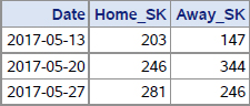
As an example, in the data set Dw.Games variables Home_SK and Away_SK identify the home team and away team, respectively. First, suppose that we are interested in games the home teams 203, 246, and 281 played in May on Saturdays. The records from Dw.Games representing these games satisfy the clause:
where Home_SK in (203,246,281) and Month=5 and DayOfWeek=7
These records look as follows:
Output 10.4 Chapter 10 Dw.Games Input for Selective Unduplication

Second, suppose that for each home team in the subset, we want to know which away team it played last – i.e., which team it played a game against in its home ballpark. In other words, we need to unduplicate the records for each key-value of Home_SK by selecting its record with the latest value of Date. For the home teams listed in the snapshot above, their most recent games, shown in bold, are those we want to keep.
Note that the file is not sorted by any of the variables. Hence, the inquiry cannot be answered simply by picking some record for each key-value of Home_SK, based on the record sequence existing in the file.
The well-beaten path most often used to solve this kind of problem is a two-step approach:
1. Sort the file by (Home_SK,Date).
2. Select the last record in each BY group identified by Home_SK.
This approach is exemplified by the program below:
Program 10.3 Chapter 10 Selective Unduplication via PROC SORT + DATA Step.sas
proc sort
data = dw.Games (keep=Date Home_SK Away_SK Month DayOfWeek)
out = games_sorted (keep=Date Home_SK Away_SK)
;
by Home_SK Date ;
where Home_SK in (203,246,281) and Month=5 and DayOfWeek=7 ;
run ;
data Last_games_sort ;
set games_sorted ;
by Home_SK ;
if last.Home_SK ;
run ;
The program generates the following output:
Output 10.5 Chapter 10 Selective Unduplication via PROC SORT + DATA Step
This method suffers from the same major flaws as using the SORT procedure for basic unduplication – i.e., the need to sort as well as dense I/O traffic. Again, using the hash object instead addresses these problem areas. Let us lay out a plan first:
1. Create a hash table keyed by Home_SK and having Date and Away_SK in the data portion.
2. Read the next record.
3. Perform the Retrieve operation using the value of Home_SK in the record as a key.
4. If this key-value is not in the table, i.e., this is the first time this value of Home_SK is seen, insert a new item with the values of Home_SK, Date, and Away_SK in the current record into the table.
5. Otherwise, if it is in the table, compare the value of Date from the record with the hash value of Date stored in the table for this Home_SK. If Date from the record is more recent, use the Update operation to replace the hash values of Date and Away_SK in the table with those from the record.
6. If there are more records to read, go to #1.
7. Otherwise, at this point the hash table contains the data being sought – i.e., all distinct values of Home_SK paired with the latest date on which it was encountered and the respective value of Away_SK. So, all we need to do now is use the Output operation, write the content of the table to an output file, and stop the program.
It can be now expressed in the SAS language:
Program 10.4 Chapter 10 Selective Unduplication via Hash.sas
data _null_ ;
dcl hash h (ordered:"A") ; ❶
h.defineKey ("Home_SK") ;
h.defineData ("Home_SK", "Date", "Away_SK") ; ❷
h.defineDone () ;
do until (lr) ;
set dw.Games (keep=Date Home_SK Away_SK Month DayOfWeek) end=lr ;
where Home_SK in (203,246,281) and Month=5 and DayOfWeek=7 ;
_Date = Date ; ❸
_Away_SK = Away_SK ;
if h.find() ne 0 then h.add() ; ❹
else if _Date > Date then
h.replace(key:Home_SK, data:Home_SK, data:_Date, data:_Away_SK) ; ❺
end ;
h.output (dataset: "Last_games_hash") ; ❻
stop ;
run ;
Since the program plan translates into its code almost verbatim, only certain technical details remain to be annotated:
❶ Coding the argument tag ORDERED:"Y" is optional and is needed only if we want the home teams in the output in their ascending order by Home_SK.
❷ Home_SK is added to the data portion of table H, so that it could appear in the output.
❸ Save the values of Date and Away_SK coming from the current record in auxiliary variables. This is necessary because if the FIND method called next succeeds, the values of these PDV host variables will be overwritten with the values of their hash counterparts. (This is an adverse side effect of the hash object design: Unlike an array, it does not allow looking at the value of a hash variable without extracting it into its PDV host variable first.)
❹ If the FIND method has succeeded for the current PDV value of Home_SK, the host value of Date is the same as its hash value. Now it can be compared with the value that came with the record and that was saved in variable _Date.
❺ If the value of _Date is more recent than that of Date, the hash item for the current Home_SK must be updated. An explicit REPLACE call is used to overwrite the hash variables with the saved values of _Date and _Away_SK.
❻ At this point, table H contains all distinct values of Home_SK coupled with the latest values of Date and the respective values of Away_SK. So, the OUTPUT method is called to dump its content to the output file.
Running the program generates exactly the same output (Output 10.4) in the same record order as the (PROC SORT + DATA step) approach if the ORDERED:"A" argument tag is used as shown above. If it were either omitted altogether or valued as "N", the output record sequence would be determined by the internal "undefined" hash table order.
An alert reader may have noticed that this program is not without flaws itself in terms of how it scales. For example, imagine that instead of the single satellite variable Away_SK we have in this simple example, there are a few dozen. It is easy to perceive that it would complicate things because:
● All these satellite variables would have to be included in the data portion of the table.
● Instead of the single reassignment _Away_SK = Away_SK in ❸, we would need as many as the number of the satellite variables.
● Though both points above could be addressed using proper code automation via the dictionary tables, the numerous variables in the data portion would increase the hash entry size accordingly. This could have negative implications from the standpoint of hash memory footprint – especially if we had a very large file with very few duplicates, which in real data processing life happens often.
The good news is that all these concerns can be addressed by using a hash index. It will be discussed in Chapter 11 as part of the discussion devoted to hash memory management.
10.3 Testing Data for Grouping
As we know, the data written from a hash table to a file always comes out grouped by the table key, whether it is simple or composite. Hence, it can be processed correctly by this key without sorting the file by using the NOTSORTED option with the BY statement.
Suppose, however, that we have a data set and would like to process it in this manner because we are suspecting (for example, from the way it looks in the SAS viewer) that the file may be intrinsically grouped by the variables we intend to use in the BY statement. If this were the case, we could save both computer resources and time by not sorting the file before doing the BY processing, particularly if the file is long and wide. So, the question arises: How can we determine, reading only the keys in question and in a single pass through the file, whether it is indeed grouped or not?
10.3.1 Grouped vs Non-Grouped
To arrive at an answer, let us observe that if a file is grouped by variable Key, it can contain one and only one sequence of same-key adjacent records for each distinct value of Key. Thus, if the values of Key in the file were:
2 2 1 3 3 3 3
then it would be grouped since the records with a given key-value are bunched together into one and only one sequence. But if the same keys were positioned in the file this way:
2 2 3 3 1 3 3
then the file would be non-grouped since now there would be two separate sequences with Key=3.
Therefore, we can check to see whether the data is grouped if, for each separate sequence of adjacent keys with the same key-value, we could determine whether this key-value has already been seen before in another sequence. To do so, each distinct key-value encountered in the process needs to be stored somewhere. The ideal container for such storage (and subsequent search) is a hash table. And in response to a question from one of our IT users, we agreed that, yes, most problems can be addressed using a hash table approach.
10.3.2 Using a Hash Table to Check for Grouping
Hence, we can devise a programmatic plan to determine if a file is grouped as follows:
1. Create a hash table keyed by the variables whose grouping we intend to check.
2. Read each consecutive sequence of same-key adjacent records one at a time.
3. At the end of each sequence, check to see if its key-value is in the table.
4. If it is not in the table, store it there and proceed to the next sequence.
5. Otherwise, if it is already in the table, we have found two separate sequences with the same key-value. Therefore, the file is not grouped, so we can flag it as such and stop reading it.
6. If the program proceeds past the last record without having been stopped, the file is grouped.
Following this plan, let us write a program to check to see if data set Dw.Runs is grouped by the composite key (Game_SK, Inning,Top_Bot) since, from a glimpse of it, it seems that it might be.
Program 10.5 Chapter 10 Testing Data for Grouping via Hash.sas
data _null_ ;
if _n_ = 1 then do ;
dcl hash h () ;
h.definekey ("Game_SK", "Inning", "Top_Bot") ; ❶
h.definedone () ;
end ;
if LR then call symput ("Grouped", "1") ; ❻
do until (last.Top_Bot) ; ❷
set dw.Runs end = LR ;
by Game_SK Inning Top_Bot notsorted ; ❸
end ;
if h.check() ne 0 then h.add() ; ❹
else do ;
call symput ("Grouped", "0") ; ❺
stop ;
end ;
run ;
%put &=Grouped ; ❼
Running the program results in the following line printed in the log:
GROUPED=1
Hence, the file is indeed grouped by the composite key (Game_SK,Inning,Top_Bot). Needless to say, by extension it is also grouped by (Game_SK,Inning) and (Game_SK) alone. Since the program follows the pseudocode almost verbatim, the annotated explanations below just fill in the gaps and underscore certain details:
❶ Key the hash table with the variables whose grouping we are tracking in the hierarchy we need. Note that the data portion is not specified as it is not needed. So the data portion variables are not defined, and therefore it contains the same variables as defined in the key portion.
❷ The DoW loop here is an ideal vehicle to read one sequence of same-key records per execution of the DATA step. Note that the key indicated in the UNTIL condition is the last component of the composite key whose grouping we are exploring.
❸ The NOTSORTED option on the BY statement ensures that the last record in the sequence read in the loop is the record whose key is simply different than the key in the next record.
❹ The end of the record sequence just read by the DoW loop has been reached. So, it is time to check if the key of this sequence is already in table H – in other words, whether any preceding sequence has had the same key. If yes, the file is not grouped, and so we act accordingly. If no, we store the key in the table as one more item.
❺ If we have found that the file is not grouped, macro variable Grouped is set to 0.
❻ If program control has reached this condition and it evaluates true, it means that after the last record was read the STOP statement has not been executed. So, the file is grouped, and macro variable Grouped is set to 1 accordingly. (Note that in this case, the DATA step is stopped not by the STOP statement but by the attempt to read from the empty buffer after all the records have been read.)
❼ In this simple example, the value of macro variable Grouped is simply displayed in the SAS log. The program can be run in a test mode to decide, depending on the resulting value of Grouped, whether to sort the file or use its inherent grouped order for BY processing with the NOTSORTED option. Alternatively, the program can be used as a step in the process to make the decision and construct code needed downstream programmatically.
This program can be easily parameterized and encapsulated as a macro. We leave it as an exercise for inquisitive readers. We did tell the business and IT users that such parameterization and encapsulation could be done in the expected follow-on project.
10.4 Hash Tables as Other Data Structures
The SAS hash object, representing in and by itself a specific data structure (i.e., the hash table), can also be used to implement other data structures. Doing so makes sense in two situations:
● The data structure the programmer needs to accomplish a task is not yet available in SAS as an encapsulated software module.
● It is available – for example, in the form of a function or procedure. However, in terms of the specific task at hand, re-implementing it using the hash object offers better functionality and/or performance.
Historically, using existing SAS data structures to implement data structures absent from the software is not uncommon. In fact, the first practically usable hash tables in SAS were implemented using a different data structure – namely, the SAS array. Conversely, now that the hash object is available, its dynamic nature, the ability to shrink and grow at run time, and search performance all offer numerous advantages in terms of using it to implement other data structures. For example:
● The original name for the hash object is an associative array. And indeed, the hash object can be viewed as an implementation of an array differing from the standard SAS array in two aspects: (a) its elements can be added to (or removed from it) dynamically at run time, and (b) it can be "subscripted" not only by an integer index but by an arbitrary composite key consisting of a number of variables with different data types.
● The hash object constructed with the argument tag HASHEXP:0 uses a single AVL binary tree. It has the property of being balanced in such a way that it can be always searched in O(log(N)) time, regardless of the distribution of its input keys. Thus, though SAS does not offer the AVL tree as a separate structure explicitly, the hash object effectively makes it readily available for use in the DATA step. Before the hash object became available, the AVL tree, if needed, would have to be coded using arrays (an exercise most SAS users would find too unpalatable to attempt).
In principle, the rich feature set of the SAS hash object provides for the implementation of just about any dynamic data structure. In this section, we will limit the discussion to the hash table operations required to implement two simple structures not yet offered as dynamic (i.e., shrink-and-grow) canned routines.
10.4.1 Stacks and Queues
Before the advent of the SAS hash object, DATA step data memory-resident structures like stacks and queues had existed in the SAS software in a certain way. In particular, a queue is implemented in the form of the LAG and DIF functions, and a stack (as well as a queue) can be organized using arrays coupled with proper custom coding. There are two main problems with these implementations:
● The number of items they store is preset at compile time. For example, the number of items available in the LAG<N> queue is statically pre-defined by its "number of lags" N; and the number of items in an array is pre-defined by its dimensions. More elements and more memory required for them cannot be allocated at run time. Likewise, their existing elements cannot be removed and memory occupied by them – released at run time. Thus, the number of lags or array dimensions must be allocated as either "big enough" or determined programmatically by an extra pass through data.
● To organize a stack or a queue with items comprising more than one variable, parallel arrays or parallel LAGs are needed. Though this is possible, it may be unwieldy, as it requires handling the variables in such parallel structures separately.
The hash object is devoid of these shortcomings, as its items can be added and removed (and the memory they occupy – acquired and released) at run time, so that any data structure based on the hash object can grow and shrink. Let us first take a very brief look at the essence of the stack and queue and their terminology.
A stack is a last-in-first-out, or LIFO, data structure. When we add an item to a stack, we perform an action called push. If we push items 1, 2, and 3 onto an initially empty stack S one at a time (from right to left below), the successive states of the stack (shown in brackets) look as follows:
S = [1] then [1 2] then [1 2 3]
When items are taken off the stack, an action called pop is performed. When we pop the stack, we surface the item we have pushed last and remove it from the stack. Hence, popping stack S=[1 2 3], for example, 2 times, we will first surface and remove item 3, and then item 2. The successive states of S after each pop will look like:
S = [1 2] then [1]
If we pop the stack one more time, item 1 will be surfaced, and the stack will become empty. Hence, a stack is useful when, after pushing items onto it one at a time, we need to access them in the order opposite to insertion. An apt example could be reading a file backward.
By contrast, a queue is a first-in-first-out, or FIFO, data structure. When we insert an item into a queue, we perform an action called enqueue. If we enqueue items 1, 2, and 3 into an initially empty queue Q one at a time (from left to right below), the successive states of the queue will look like so:
Q = [1] then [2 1] then [3 2 1]
When items are taken from the queue, an action called dequeue is performed. By dequeueing, we surface the item queued first and remove it from the queue. Thus, if we dequeue queue Q above 2 times, we will surface and remove item 1, and then item 2; and the successive states of Q after each dequeue will look as follows:
Q = [3 2] then [3]
If we dequeue once more, item 3 will be surfaced, and the queue will be emptied. A good example of the dequeuing order could be reading a file forward.
Implementing a stack or a queue based on a hash table in formal accordance to the rules above is conceptually simple:
● Have a hash table as a container for a stack or a queue and pair it with a hash iterator.
● To either push an item onto the stack or queue the queue with an item, simply insert it into the table. Do it as many times as necessary before an item needs to be either popped off the stack or dequeued from the queue.
● To pop an item off the stack, access the logically last item, retrieve its content, and remove it from the table.
● To dequeue an item from the queue, access the logically first item, retrieve its content, and remove it from the table.
Note that thanks to the fact that the hash table facilitates access to its items from both ends, the same hash table can be used both as a stack and a queue. The difference between the two materializes only when an item is surfaced: To use the table as a stack, we pop the item added to the table most recently; and to use it as a queue, we dequeue the item added least recently. Let us now see how it can be implemented programmatically, first for a stack and then for a queue.
10.4.2 Implementing a Stack
The program presented below does the following:
● Creates a hash table as a container for a stack.
● Pushes 3 items on the stack.
● Pops 1 item off the stack.
● Pushes 2 new items.
● Pops 2 items.
● After each action above, writes a record to an output demo file showing the PDV data value pushed or popped and the items on the stack.
Note that the italicized lines of code below are unrelated to the stack actions and serve only to render the demo output.
Program 10.6 Chapter 10 Implementing a Hash Stack.sas
data Demo_Stack (keep = Action PDV_Data Items) ;
dcl hash h (ordered:"A") ; ❶
h.defineKey ("Key") ;
h.defineData ("Key", "Data") ;
h.definedone () ;
dcl hiter ih ("h") ; ❷
Data = "A" ; link Push ; ❸
Data = "B" ; link Push ;
Data = "C" ; link Push ;
link Pop ;
Data = "D" ; link Push ;
Data = "E" ; link Push ;
link Pop ;
link Pop ;
stop ;
Push: Key = h.num_items + 1 ; ❹
h.add() ;
Action = "Push" ;
link List ;
return ;
Pop: ih.last() ; ❺
rc = ih.next() ;
h.remove() ;
Action = "Pop" ;
link List ;
return ;
List: PDV_Data = Data ; ❻
Items = put ("", $64.) ;
do while (ih.next() = 0) ;
Items = catx (" ", Items, cats ("[", Key, ",", Data, "]"));
end ;
output ;
return ;
run ;
Let us dwell on a few points in the program that might need explanation:
❶ Hash table H created to hold the stack/queue (a) is ordered, (b) allows no same-key items, and (c) has its key also added to the data portion. The sole reason for this triple arrangement is the "classic" requirement that after an item is popped, it must be removed. This is because to remove only the first or last item – and not any other item – its key-value must be unique and we need to know it. But to retrieve it using the hash iterator alone without extraneous bookkeeping (which is the intent), the key must be also defined in the data portion. (As we will see later, if the removal requirement is dropped, none of the three measures is needed.)
❷ Hash iterator IH coupled with table H is declared in order to access the first or last item regardless of their keys.
❸ This and the next 7 lines of code call the corresponding LINK routines to: (1) push 3 items on the stack, (2) pop 1 item, (3) push 2 new items, (4) pop 2 items.
❹ The Push routine first creates a new unique key by adding 1 to the value of the hash attribute H.NUM_ITEMS. Then a new item is inserted by calling the ADD method accepting the new value of the key and the current PDV value of host variable Data.
❺ The Pop routine performs the Enumerate All operation by using the iterator to access the last item. (Since the item with the highest key is always the one pushed onto the stack last, the routine thus conforms to the LIFO principle.) The hash value of Data from the last item retrieved into the PDV host variable Data by the LAST method call is the value the pop action surfaces (and it will also be used in the REMOVE call later). The call to the iterator method NEXT moves the iterator pointer out of the table, thus releasing its lock on the last item, so that it can be removed. The call is assigned to avoid log errors because it is guaranteed to fail: if the iterator dwells on the last item, there is no next item to enumerate. Finally, the Delete operation is performed by calling the REMOVE method which accepts the PDV value of Key the LAST method extracted earlier.
❻ The LINK routine List called after each stack action assembles the [Key , Data] value pairs from the currently available hash (stack) items into a long single variable Items, and outputs the corresponding demo record. Its function is purely auxiliary, and it is unrelated to the stack actions.
Running the program generates the output below. Note that in the Items column, the rightmost and leftmost items represent the top and bottom of the stack, respectively.
Output 10.6 Chapter 10 Using a Hash Table as a Stack

The output confirms that in the program above, the behavior of hash table H conforms with the LIFO principle and thus operates as a stack, i.e.:
● After every Push action, the current value of PDV host variable Data ends up at the top of the stack as the value of hash variable Data in the newly inserted hash item.
● Conversely, after every Pop action, the host variable Data receives the value of hash variable Data from the item at the top of the stack, after which the item is removed.
10.4.3 Implementing a Queue
Now let us consider a very similar program for organizing and operating a queue:
Program 10.7 Chapter 10 Implementing a Hash Queue.sas
data Demo_Queue (keep = Action PDV_Data Items) ;
dcl hash h (ordered:"A") ;
h.defineKey ("Key") ;
h.defineData ("Key", "Data") ;
h.definedone () ;
dcl hiter ih ("h") ;
Data = "A" ; link Queue ;
Data = "B" ; link Queue ;
Data = "C" ; link Queue ;
link DeQueue ;
Data = "D" ; link Queue ;
Data = "E" ; link Queue ;
link DeQueue ;
link DeQueue ;
stop ;
Queue: Key + 1 ; ❶
h.add() ;
Action = "Queue " ;
link List ;
return ;
DeQueue: ih.first() ; ❷
rc = ih.prev() ;
h.remove() ;
Action = "DeQueue" ;
link List ;
return ;
List: PDV_Data = Data ;
Items = put ("", $64.) ;
do while (ih.next() = 0) ;
Items = catx (" ", Items, cats ("[", Key, ",", Data, "]")) ;
end ;
output ;
return ;
run ;
Its output looks as follows:
Output 10.7 Chapter 10 Using a Hash Table as a Queue

The program and output for the queue look quite similar to those for the stack. However, there are a few significant distinctions (in the program, they are shown in bold):
❶ The queue action is different from push in that a new item is queued into the back of the queue. Thus, we want each newly queued item at the bottom of the table. This is done by incrementing the key and inserting the item being queued using the ADD method.
❷ The dequeue action is similar to the pop action of the stack. However, instead of retrieving the Data value from the last item (i.e., the back of the queue), it retrieves it from the first item (i.e., the front) and then removes it. To do so, the iterator lock on the first item needs to be released first. This is done by calling the PREV method which moves the iterator pointer out of the table, thus releasing the first item.
10.4.4 Using a Hash Stack to Find Consecutive Events
As a practical example, suppose that we want to find, from the content of file Dw.AtBats, the latest 6 games in the season where 4 or more back-to-back home runs were scored, along with the actual back-to-back home run count. This is a typical LIFO requirement, meaning that we need a stack.
The inquiry stated above can be answered by making use of the fact that the records in Dw.AtBats are entered chronologically. Therefore, if a series of 4 or more records marked as Result="Home Run" is both preceded and followed by a different value of Result, we have identified a back-to-back event we are looking for. For example, let us take a look at this group of consecutive records from the file. (The column From_obs is not a field in the file; it just indicates which observation in Dw.AtBats the records shown below come from.)
Output 10.8 Chapter 10 Dw.AtBats Record Sample with Back-to-Back Events

Above, the records 54227-54250 and 54252-54253 represent consecutive back-to-back events. In particular, the records where Result="Home Run" represents a back-to-back, 4-home-runs event. Every time we encounter such an event, we can push the corresponding item on the stack. After the entire file has been processed, we can simply pop 6 items off the stack and output their contents to a file.
Let us now program it in SAS. Note that this program incorporates coding for the stack without calling LINK routines and deviates from the stack demo program above in some details to better fit the specific task and make use of specific data. However, the general scheme is kept intact.
Program 10.8 Chapter 10 Using a Hash Stack to Find Consecutive Events.sas
data StackOut (keep = Game_SK Result Count) ;
if _n_ = 1 then do ;
dcl hash stack (ordered:"A") ; ❶
stack.defineKey ("_N_") ; ❷
stack.defineData ("_N_", "Game_SK", "Result", "Count") ;
stack.defineDone () ;
dcl hiter istack ("stack") ; ❸
end ;
do until (last.Result) ; ❹
set dw.AtBats (keep = Game_SK Result) end = LR ;
by Game_SK Result notsorted ;
Count = sum (Count, 1) ;
end ;
if Result = "Home Run" and Count => 4 then stack.add() ; ❺
if LR ;
do pop = 1 to 6 while (istack.last() = 0) ; ❻
output ;
rc = istack.next() ;
stack.remove() ;
end ;
run ;
❶ Create a hash table Stack to be used as a stack – ordered ascending by its key.
❷ Stack is keyed by the automatic variable _N_. The idea is to key the table by a variable that naturally ascends along with each new event of 4 back-to-back home runs; and _N_ fits the purpose by its very nature of invariably ascending with each execution of the DATA step. Then _N_ is added to the data portion to facilitate the removal of every popped item via the REMOVE method.
Note that using _N_ as a key (rather than Key in the demo program) takes advantage of the intrinsic DATA step mechanics and rids us of the extra necessity to use the NUM_ITEMS attribute in the push action.
❸ Pair table Stack with a hash iterator instance needed to facilitate the stack pop operation later on.
❹ This DoW loop uses the NOTSORTED option to isolate each series of consecutive records with the same value of Result within Game_SK into a separate DATA step execution. This way, after the DoW loop has finished iterating, the PDV value of Result corresponds to its value in the series the loop isolates; and the value of Count indicates the number of records in the series – or, in other words, the number of times the DoW loop has iterated.
❺ The DoW loop has finished iterating over the current same-key series. If it is a series of home runs and its length is 4 or greater, push a new item on the stack S. Note that, unlike Key in the demo program, _N_ does not have to be incremented before calling the ADD method as a key, as it gets a proper ascending unique value automatically.
❻ At this point, all input records have been processed, so we need to pop the required number of items off the hash stack. Including the LAST iterator method call in the WHILE condition ensures that if the stack is empty – meaning that no 4 or more consecutive home runs have been scored – program control exits the DO loop without executing its body even once, and so no output record is written out. Otherwise, the call retrieves the values of the data portion hash variables into their PDV host counterparts, the next record is output; and the rest of the requisite pop action activities are performed. If the number of 4 or more back-to-back home run chains N< 6, the loop stops after its Nth iteration and having output N records according to the number of items N on the stack. (The value of 6 is chosen arbitrarily just as an example; any other value can be used.)
Running the program, we get the following output:
Output 10.9 Chapter 10 Latest Games with 4 or More Back-to-Back Home Runs


Since the stack is popped in the LIFO manner, the latest games where 4 or more consecutive home runs were scored come in the output first, as should be expected.
Note that we have provided alternative examples of consecutive events in section 8.2.3.5 “Determining the Distribution of Consecutive Events” and in section 9.4 “Consecutive Events.” Those examples created a distribution of the number of consecutive events. Using a hash stack is an alternative approach and Program 10.8 could be modified to create a distribution in addition to creating a list of occurrences of multiple events. This example also allowed us to point out to our users that one of the great things about SAS is that there are multiple different ways to solve virtually any given problem.
10.5 Array Sorting
Sorting an array may appear as a largely academic exercise. Yet, judging from the number of inquiries about the ways to do it on various SAS forums, it must have a number of practical applications. However, custom coding an efficient array sorting routine is not an exercise for faint-hearted. Before the advent of the canned array sorting routines, some SAS programmers had successfully endeavored to code their own custom routines based on well-known algorithms, such as the quick sort or radix sort. Currently, the efficient call routines SORTN and SORTC are offered to do the job. However, they are not without shortcomings; specifically:
● They are data type specific (unlike the SORT procedure, for example).
● They are sorted only in ascending order.
● They offer no options to handle duplicate keys.
● They are not suited for sorting parallel arrays in sync.
10.5.1 Using a Hash Table to Sort Arrays
The Order hash object operation can be easily used to address these problem areas. The basic scheme of using the hash object to sort an array is quite simple:
1. Load the key and satellite elements from the array(s) into a hash table ordered ascending or descending.
2. Unload the hash table back into the array(s).
In a nutshell, that is it. Now let us look at some implementation details. Suppose we have 3 arrays valued as follows:
array kN [9] ( 7 7 7 7 5 5 5 3 3 ) ;
array kC [9] $1 ('F' 'E' 'F' 'E' 'D' 'C' 'D' 'A' 'B') ;
array dN [9] ( 8 6 9 7 4 3 5 1 2 ) ;
The elements of arrays kN and kC represent a composite key, by which they have to be sorted into ascending or descending order. As a result, the elements of array dN should be permuted in sync with the new index positions of the elements of the key arrays. Provisions should also be made to eliminate all duplicate-key elements, except for the first-in or last-in, if necessary. For instance, if the arrays are sorted ascending by (kN,kC) and duplicate keys are allowed, their resulting array values would look like this:
kN: 3 3 5 5 5 7 7 7 7
kC: A B C D D E E F F
dN: 1 2 3 4 5 6 7 8 9
Or, if we need to sort in descending order and only the first element with a duplicate key must be kept, they should look as follows:
kN: 7 7 5 5 3 3 . . .
kC: F E D C B A
dN: 8 6 4 3 2 1 . . .
Making use of the hash object, we can thus write the following simple array-sorting program:
Program 10.9 Chapter 11 Array Sorting via Hash
%let order = A ; * Sort: A/D (Ascending/Descending ; ❶
%let dupes = N ; * Dups: Y/N (Yes/No) ;
%let which = L ; * Dupe to select: F/L (First/Last) ;
data _null_ ;
array kN [9] ( 7 7 7 7 5 5 5 3 3 ) ;
array kC [9] $1 ('F' 'E' 'F' 'E' 'D' 'C' 'D' 'A' 'B') ;
array dN [9] ( 8 6 9 7 4 3 5 1 2 ) ;
if _n_ = 1 then do ;
dcl hash h (multidata:"Y", ordered:"&order") ; ❷
h.defineKey ("_kN", "_kC") ; ❸
h.defineData ("_kN", "_kC", "_dN") ;
h.defineDone () ;
dcl hiter hi ("h") ; ❹
end ;
do _j = 1 to dim (kN) ;
_kN = kN[_j] ; _kC = kC[_j] ; _dN = dN[_j] ; ❺
if "&dupes" = "Y" then h.add() ; ❻
else if "&which" = "F" then h.ref() ; ❼
else h.replace() ; ❽
end ;
call missing (of kN[*], of kC[*], of dN[*]) ; ❾
do _j = 1 by 1 while (hi.next() = 0) ; ❿
kN[_j] = _kN ; kC[_j] = _kC ; dN[_j] = _dN ;
end ;
h.clear() ;
put "kN: " kN[*] / "kC: " kC[*] / "dN: " dN[*] ;
run ;
If run with the parameterization as shown above, the DATA step will print the following in the log:
kN: 3 3 5 5 7 7 . . .
kC: A B C D E F
dN: 1 2 3 5 7 9 . . .
Let us see how hash object operations fit in this code to accomplish the task and how its logic flows:
❶ The %LET statements provide parameterization useful to encapsulate the routine in a macro if need be.
❷ Hash table H is created with MULTIDATA always valued as "Y" (i.e., this value is not parameterized on purpose). Duplicate keys are handled later via choosing a specific table-loading method. The _N_=1 condition is just a precaution in case the sorting routine is to be also performed for _N_>1, such as for new observations or new BY groups. Compare this with the CLEAR method call in ❿ below.
❸ The key and data portions of H defined with temporary variables whose PDV host variables are created downstream by assignment. (See item ❺.)
❹ We need a hash iterator linked to table H to enumerate its sorted data and put it back into the arrays. So, a hash iterator named HI is declared here.
❺ Forward-scan the arrays in a DO loop. Assign each element to the respective temporary PDV variable. The assignment statements both value them and make them take on the data type (numeric or character) corresponding to that of the respective array. This way, the hash variables get their host variables in the PDV at compile time and inherit the proper data types (according to the arrays they relate to) from them at run time.
❻ If unduplication is not required, call the ADD method to perform the Insert operation. Because of MULTIDATA:"Y" it will insert a new item from the array elements with the current _j index regardless of the items already in the table.
❼ Otherwise, if unduplication is required and the first duplicate for the current key must be kept, call the REF method. It automatically does what is needed because it inserts an item only if the key it accepts is not already in the table.
❽ If unduplication is required but the last duplicate for the current key must be kept, perform the Update All operation by calling the REPLACE method. It works as required here because we are attempting to add one item at a time. So, every time REPLACE is called, it can find only one item with the current key previously inserted in the table and keeps repeatedly updating it with the new values of dN[_j]. Thus, in the end, each item in the table will have the last dN[_j] value encountered for this item's key. Q.E.D.
❾ Just in case unduplication is requested, populate the arrays with missing values. This way, all duplicate-key elements being kept in the arrays will be shifted to the left, and the slack to the right will be filled with nulls.
❿ Perform the Enumerate All operation to retrieve the data portion values from each item into their PDV host variables and assign the latter to the corresponding elements of the corresponding arrays. After this is done, the CLEAR method is called to empty the hash table just in case the sorting routine is to be repeated – for example, in other executions of the DATA step for _N_>1, such as for new observations or new BY groups. The PUT statement is used merely to display the final state of the arrays in the SAS log.
Note that this sample program provides a basic framework for sorting arrays using the hash object. It can be further tailored to your particular needs depending on the circumstances and encapsulated accordingly. For example, a parameter can be added to indicate which arrays constitute the composite key and which constitute the data elements to be permuted in accordance with the new positions of the key-value.
10.6 Summary
The SAS hash object can be used to provide a wide range of data structures and, as shown in this chapter, it can be integrated with other SAS functionality to do that. There are any number of additional examples that are possible. Our IT users were quite pleased with the examples presented here and told us that should a follow-on project be approved, they would likely request additional examples.