
Classical Project Time Control Techniques
Overview
Although projects have been managed since the dawn of civilization, but the terms, concepts, and techniques of project management only began to be developed around 1910s when one of the most common project scheduling tools, the Gantt bar chart, was popularized. Since then, various techniques of project management have been developed, including many that are used for controlling the time of projects. In Chapter 6, the PCIM project control methodology put forward several of these project time control techniques to support the good practices contained in the PCIM project control methodology for the project control steps of planning, monitoring, reporting, and analyzing. The most common project time control techniques are explained in this chapter following a discussion on the concept of project time control below.
Project Time (Schedule) Control
The control of time is also often referred to as schedule control. This process involves determining the status of the project schedule, determining if changes have occurred or should, and implementing and managing schedule changes. It is important to apply time control on projects because, for the outcome of a project to be beneficial, it must be obtained within timescales and Turner (2006) argued that there are at least three ways in which time can have an impact:
• When the output only has the desired benefit at a certain time, for example a sporting event such as the 2022 men’s football world cup in Qatar has a defined time at which the event must start, if the project is late all the benefit is lost.
• Sometimes the output of a project only has the desired benefit over a limited market window. An example could be the launch of a seasonal product.
• Due to the time value of money, the later a project is delivered the more it costs, and so value is eroded.
The Essential Element of Time Control: The Project Schedule
The project schedule is an essential prerequisite for time control of projects. It is one of the most important tools in the control of the time plan of a project. This is not surprising because first and foremost planning is an important technique of project management and the project schedule is an important project time planning tool. The master schedule for a project shows all the project stakeholders the start date and the completion time of a project (See section titled “Visual Representation of Project Duration” in Chapter 3, for more information on different types of project schedules used in practice). The master schedule also details the important phases of work, their duration, and a breakdown of major work to be done during each stage. The project schedule is therefore an important measure of the progress being made in relation to the completion date during the delivery of the project. If used factually and accurately, analysis of the project schedule would show if the project is ahead of schedule, on schedule, or behind schedule. The project schedule can therefore be used to measure and control time progress, and if things were not going according to plan, the project team would need to find a remedy for the situation. The following sections discuss some key issues relating to the project schedule.
Description and Purpose of the Project Schedule
A schedule is the conversion of a project plan into the constituent activities with their associate completion timeline, which then creates a timetable upon aggregation. It is a series of dates against the elements in the work breakdown structure, which record when the project management team forecast the work will occur and, through monitoring, when the work eventually happens. The project schedule records the planned and actual start date, finish date, and duration of each work element. It may also record whether there is any flexibility when each element may start without delaying the completion of the project, which is called the float (discussed later in the chapter).
The aim of work scheduling is to achieve an economic balance between the utilization of resources and the cost of work in progress. This means that the scheduled time of a project is linked to the cost incurred as has been noted by the PCIM project control methodology. Scheduling work to be completed rapidly would usually have a high-cost implication due the use of additional resources or manhours than planned or working overtime, which will need to be paid for. While scheduling work to progress too slowly will usually also incur a higher cost due to spending more time in delivering the project. Therefore, the project schedule helps achieve the right balance based on the objectives of the project owner and available resources for the project. The project schedule helps to highlight the major elements of the time and progression plan of a project and communicate these to the stakeholders. The purposes of a project schedule are as follows:
• Presents the activities to be delivered on a project;
• Shows the sequence of the project activities;
• Includes the interdependencies of project activities;
• Includes the key project milestones;
• Shows key dates;
• Shows the milestone dates;
• Presents the operational approach and logic for delivering the project;
• Used to deliver the project;
• Provides a means of monitoring the progress of deliverables within the execution phase of the project;
• Serves as the basis for monitoring and controlling project activity.
Types of Schedule
The main approaches to scheduling are bar charts (Gantt charts), milestone charts, and networks such as arrow diagram method (ADM), precedence diagram method (PDM), program/graphical evaluation, and review techniques and linear scheduling such as line of balance (LOB) have been argued as an approach as well.
From the aforementioned, it is apparent that schedules can be classified broadly as non-network-based schedules and network-based schedules.
Non-Network-Based Schedules
These types of schedules include milestones and bar charts. The most popular non-network-based schedule is the bar chart or Gantt chart; it is one of the oldest and simplest forms of the project schedule. The Gantt chart was named after the famous management consultant Henry L. Gantt (1861–1919) (Seymour and Hussein 2014). Despite its age, the Gantt chart is still an important and popular tool in 21st century project management. The Gantt chart technique is discussed later in this chapter.
Network-Based Schedules
Network-based time control techniques sequence the activities required in the implementation of a project diagrammatically as a network showing the interdependencies and interrelationships of these activities. The planning data in the network is linked through the logic that defines the relationships between the activities. Therefore, changes can be made in the data relating to individual activities (i.e., the duration, the resources, etc.) or changes can be made in the logical relationships between activities and the consequences recalculated and represented.
Milestone Technique
One of the simplest techniques for controlling projects is the milestone technique. This is basically a time scheduling technique, which allows important deadlines in a project to be highlighted by specific points in time, called milestones. These activities are usually at the beginning or end of a phase or stage and are used for monitoring purposes throughout the life of the project. A milestone schedule will show the key events of a project (the milestones), on a diagrammatical representation of the project’s delivery sequence forecast from start to finish. The key to helpful use of milestones techniques is selectivity, that is, choosing only a few key events as milestones. The disadvantage of the milestone technique is that it does not clarify the dependencies associated with activities or tasks.
Milestone Slip Chart
A milestone slip chart is a type of progress report as shown in Figure 7.1. For projects, it can be developed by plotting the milestones associated with a project on a grid on a periodic basis to indicate the planned date for that milestone.
How the milestone slip chart is used in practice is described below.
• Week “0”: In Figure 7.1, the start of the project is a point “0.” In the baseline schedule, milestone A is due to occur in week 2, milestone B in week 5, and milestone C in week 7.
• Week 1: After the first week, the three milestones, A, B, and C are on track.
• Week 2: However, by the end of week two, they have fallen behind their planned date by one week.
• Week 3: At the end of week three, A is completed but one week later than planned and the other milestones are still behind their planned date by one week.
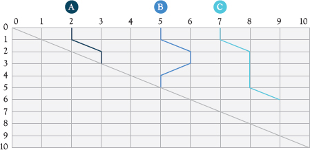
Figure 7.1 Example of a milestone slip chart
• Week 4: In week four, B is back on track but C is still behind its planned date by one week.
• Week 5: In week five, B is completed on time.
• Week 6: However, in week six, C is now behind its planned date by an additional week.
The advantage of the milestone slip chart is its simplicity and ability to present a high-level view of progress using the key milestones dates of the project transferred from the detailed project schedule.
Graphical Analysis (Bar Charts)
Bar charts as previously mentioned are often called Gantt charts after Henry Laurence Gantt, an American engineer and management consultant who popularized them during the First World War. During this period, Gantt worked with the U.S. Army on a method for visually portraying the status of the munitions’ programs. He realized that time was common denominator to most elements of a project’s delivery schedule and that progress could easily be assessed by viewing each element’s status with respect to time (Nicholas 2020).
Although the bar charts are popularly named after Gantt, it was Karol Adamiecki, a Polish engineer and economist researcher who first developed a novel means of displaying interdependent processes to enhance the visibility of production schedules in 1896. However, his works were published in Polish and Russian languages and were not popular in the English-speaking world where Gantt published on a similar technique in 1910 and 1915. Therefore, this technique is referred to in English by Gantt’s name. Gantt charts were utilized in many major American First World War infrastructure projects including the Hoover Dam, which as concluded by Seymour and Hussein (2014), popularized it and contributed to its widespread adoption. Figure 7.2 shows an example of a bar chart used to schedule a project. The structure of the Gantt chart is as follows:
• A horizontal timescale to show activity duration
• A vertical list of activities
• A horizontal line or bar for each activity
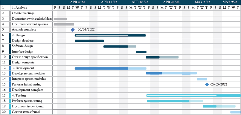
Figure 7.2 Example of a bar chart
In addition to these, bar charts show the sequence of activities to be delivered on a project graphically using the dependencies and interrelationship between or among activities. They can also show schedule dates, milestones, key dates, and can be used to show current progress status of the project.
Advantages of Bar Charts
• Bar charts are easy to develop for projects and update as the project progresses.
• They can be used to provide a high-level overview of a project’s timetable including dependencies and overlaps.
• Stakeholders find them more straightforward to understand.
• They can be used to present the timelines of multiple projects in a noncomplex format, then used to monitor and control the progress of the multiple projects.
• The critical path is produced before the floats are known unlike some other methods, where the floats must be calculated first before the critical path can be seen. The advantage of this is that the scheduler or planner can know immediately whether the project time is within the specified limits and adjust the critical activities without bothering with the noncritical ones (Lester 2017).
Limitations of Bar Charts
• One of the disadvantages of the Gantt chart, according to Nicholas (2020), is that it does not show explicitly the interrelationships among work elements, that is, it does not reveal the effect of one work element falling behind schedule on other elements.
• Bar charts provide only a vague description of how the entire program or project reacts as a system; they do not show the interdependencies of the activities and therefore do not represent a “network” of activities. Since the relationship between activities is crucial for controlling project costs, bar charts have little predictive value (Kerzner (2017).
• Knowing the status of project activities gives no information at all about overall project status because only one activity’s dependence on another is shown.
• Bar charts are often maintained manually. This is usually not a problem for small projects but onerous for large projects, consequently causing lethargic updates and results in the bar charts becoming outdated.
• Bar charts, according to Kerzner (2017), do not show the uncertainty involved in performing each activity and, therefore, do not lend themselves readily to sensitivity analysis. For instance, answering questions like: What is the shortest time or longest time an activity might take? What is the average or expected time to complete an activity?
• The use of percentage completion mostly used for progress monitoring on bar charts usually leads to subjectivity and confusion as it does not provide the information on whether the performance dimension relates to the schedule dimension or the cost dimension. Therefore, it becomes impossible to judge what percentage of activity is truly complete.
LOB Method
The LOB method originated in the Goodyear Company in the 1940s and was developed by the U.S. Navy during the Second World War. The method is used when a project consists of blocks of the same or similar work or repetitive activities. It is often used where the same activities are performed by the same team; hence it is also referred to as the linear scheduling method. The LOB (see Figure 7.3) compares time and location or sequence number of repetitive elements. The horizontal axis plots time, while the vertical axis plots location or distance along the length of a project. Individual activities are plotted separately, resulting in a series of diagonal lines. The slopes of the diagonal lines represent the planned rate of progress at any time of any activity. The completion time for each activity is a function of the rate of progress and the amount of work to be undertaken.
The production goal is determined by the scope of the project. Based on the requirements of the users, the delivery schedule is produced; thereafter the production goal can be expressed in terms of the objective chart. The time required to produce the unit is calculated and the completion times and lead times of each activity are determined after which the progress chart is drawn. The horizontal scale corresponds to the number of control points in the production plan. The vertical scale corresponds to the cumulative quantities of the production units. The LOB is the level of the cumulative qualities, which must be available at any specific delivery time. The basis of the technique, as noted by Harris, McCaffer, and Edum-Fotwe (2013), is to find the required resources for each stage or operation so that the subsequent stages are not interfered with while achieving the target output.
Advantages and Disadvantages of the LOB Method
As would have been noted earlier, the main advantage of using the LOB is that it is a very useful control technique that can be used for repetitive projects, which means it may be unsuitable for nonrepetitive projects. Scheduling techniques utilizing network analysis are usually employed for planning one-off projects, be it a construction project, a manufacturing operation, a computer software development, or a move to new premises. However, when the overall project consists of several identical operations, each of which may be a subproject, then the use of the LOB technique may be advantageous. In addition to this, the advantages and disadvantages of the LOB technique include the following.
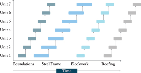
Figure 7.3 Example of a LOB chart
• It is a simple process that can be implemented manually.
• It provides a graphical interface that enables users to identify and interpret the production rates, durations, and relationships between repeating tasks quickly (Tokdemir, Erol, and Dikmen 2019).
• Each line on a LOB shows the rate of progress of an activity, which neither bar charts nor network schedules can do.
• It presents clearly the quantity of work taking place in certain areas and at a specific time of the project.
• It serves as a midway between bar charts and networks from a complexity viewpoint. Therefore, the LOB is easier to develop than a network schedule, but it is more rigorous than a bar chart.
• It facilitates the incorporation of the learning effect during scheduling, which results in a gradual reduction in the labor-hours requirements of repeating tasks (Tokdemir et al. 2019).
• It can also be used for nonrepetitive activities, especially when there is a need to evaluate the best combination of individual progress rates.
Disadvantages
• The disadvantages include the disadvantage associated with non-network-based techniques such as the bar chart as described in the section titled Non-Network-Based Schedules” earlier in this chapter.
• A major difficulty in LOB is determining the buffer interval (the buffer is the duration by which an activity could be delayed without affecting the overall project duration), which sometimes can best be found out when the production rates of adjacent activities are known.
• Updating the LOB once a project has started can be difficult and become quickly unclear, especially if the actual rates of construction prove to be different from those planned (Harris, McCaffer, and Edum-Fotwe, 2013).
Precedence Diagramming Method
The precedence diagramming method (PDM) grew out of the arrow networks to overcome some of the arrow network faults. In the PDM, three different notations are available to show a variety of start-to-finish relationships to fit any type of activity. This gives more flexibility to notation when developing logic diagrams. The PDM shows the activity number in the block, which then leaves more room to describe the activity in greater detail.
The PDM allows the overall project to be presented visually as a precedence diagram, known as the overall precedence. It can also be used to show part of the project to create partial precedence diagrams. A precedence diagram is created using graphical methods. The most visually imposing part of a PDM is the node. The node describes the connection point and an arrow of a presentation element to indicate the relationship between two nodes. The PDM (see Figure 7.4) is made up of processes (activities with established earliest and latest start and end points), event (defined and documented state in a project), and relationship (dependencies between individual processes).
Advantages of PDM
• The arrow network scheduling procedures assume a strict sequential relationship upon which the start of an activity is predicated upon the completion of its immediate predecessors, that is, a finish-to-start (FS) relationship. However, the PDM is not this strict and can handle the scheduling of tasks that can start when their predecessors are completed partially (but not fully).
• Besides the usual FS relationships, PDM permits the relationships of start-to-start, finish-to-finish, and start-to-finish and has the ability to show when an activity can start before the preceding one is completed.
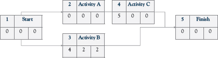
Figure 7.4 Example of a precedence diagram
• The PDM allows dependencies between activities and the effects of changes to be quickly recognized.
• It helps in the identification of relationships and dependencies among activities to identify easily any missing task.
• It allows the identification of critical processes and activities, which can then be presented as a critical path.
Limitations of PDM
The drawbacks of the PDM are as follows:
• First, because of the lead and lag requirement, activities may appear to have a float when they really do not.
• Second, as highlighted by Meredith, Shafer, and Mantel (2021), it is susceptible to reverser critical phenomenon where the critical path enters the completion of an activity through a finish constraint, continues backward through the activity, and leaves through a start constraint. The consequence of this is that increasing an activity time may actually decrease the project completion time inadvertently.
Critical Path Method
The critical path method (CPM) was almost simultaneously developed in 1958 by the Central Electric Generating Board in England and the joint effort of the U.S. Navy and one of its contractors (Du Pont) in the United States (Lester 2017). CPM includes a mathematical procedure for estimating the trade-off between project duration and project cost and, as asserted by Nicholas (2020), the CPM features the analysis of reallocation of resources from one job to another to achieve the greatest reduction in project duration at the least cost. The fundamental purpose of CPM is to enable the identification of the minimum overall project duration. The critical path of a project is the longest duration logically required to complete a project; with any delay in activities on this critical path will delay the completion date of the project. It is the path where all the activities on it have zero float (float is the amount of time an activity can be delayed before it begins to delay the project; it is the amount of time between the completion of an activity and its succeeding activity). The relationships between activities in a critical path are shown using networks. A network typically contains the nodes that contain information about the activities and arrows that are used to show the logical relationships between activities such as finish-to-start, start-to-start, finish-to-finish (see Figure 7.5).
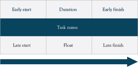
Figure 7.5 Node and arrow in a CPM network
Uses and Advantages of the CPM
• The CPM has been used widely for project scheduling, helping managers to guarantee the timely and on-budget completion of projects by identifying the most critical elements of the project.
• CPM shows the activities and their outcomes as a network diagram and enables the identification of activities that can be delivered simultaneously.
• CPM provides useful information for the project, such as the critical path(s) and free and total float, which are essential for the efficient planning of a project.
• It can aid in the optimization of the project through the determination of the overall project duration.
• It can facilitate management by exceptions through a focus on critical and near-critical activities, especially on projects that are large and complex.
• CPM establishes the dependencies among activities of a project and aids the scheduling of individual activities.
Limitations of CPM
• CPM assumes that there are unlimited resources for the execution of the activities, but in real projects, resources are not unlimited. Thus, scheduling without considering resource constraints gives unreliable schedules.
• Because the CPM caters to the scheduling of resource allocation, it is not suitable for scheduling resource-constrained projects.
• The critical path is not always clear and it can sometimes be difficult to estimate the activity completion time in a multidimensional project.
• Identifying and determining a critical path can be difficult when there are many other similar duration paths in the project.
• The CPM network can become very complicated on big projects and not straightforward for all project stakeholders to comprehend.
• The critical path needs to be always calculated accurately, therefore requiring a lot of time and effort; for big projects with long durations, it requires the use of software to monitor the schedule.
• CPM can become ineffective and difficult to manage if it is not well-defined and stable.
• Sudden changes in the delivery plan of the project during execution can be problematic when using the CPM, that is, it can be challenging to redraw the entire CPM chart if the plan of the project suddenly deviates from the original.
Program Evaluation and Review Technique
The program evaluation and review technique (PERT) was originally developed in 1958 to meet the needs of the “age of massive engineering” where the techniques of Gantt were not sophisticated sufficiently. The Special Projects Office of the U.S. Navy, concerned with performance trends on large military development program, introduced PERT on its Polaris Weapon System in 1958. According to Kezner (2017), this was after the technique had been developed with the aid of the management consulting firm of Booz, Allen, and Hamilton as a way of handling uncertainties in the estimating activity times. PERT has since spread rapidly throughout almost all industries. It adopts the critical path like the CPM described earlier to compute expected project duration, early and late times, and floats. Although, as highlighted by Nicholas (2020), PERT and CPM are similar, they were developed independently in different problem environments and industries. PERT is event-oriented (i.e., the event labels go in the nodes of the diagram) and has typically been used in aerospace and research development projects for which the time for each activity is uncertain. PERT is mostly applied to projects characterized by uncertainties; therefore, its focus is probabilistic and applies statistical treatment to the possible range of activity time duration as described in the section below.
PERT Time Estimating
PERT networks originated in projects characterized by uncertain times for activities as noted above. This problem of uncertain times was dealt with by requiring three-point probabilistic time estimates for each activity, that is:
• The most likely activity time;
• The optimistic activity time, which is the shortest time that might be achieved 1 percent of the time such an activity was carried out;
• The pessimistic activity time, which is, the longest time that would be exceeded only 1 percent of the time such an activity was carried out.
The range between the estimates provides a measure of variability, which permits statistical inferences to be made about the likelihood of project events happening at a time (Nicholas 2020). This procedure differentiates PERT from the CPM, which calculates the critical path and slack times (float) only using best estimates of activities. As shown in Figure 7.6, the three estimates are related in the form of a beta probability distribution with parameters O (optimistic time) and P (pessimistic time) as the end points, and M (most likely time) the most frequent value. The beta distribution was chosen by the originators because it is unimodal, has finite end points, and is not necessarily symmetrical, properties that seem desirable for a distribution time. Based on this distribution, the mean or expected time (te) and variance (V) of each activity are computed with three estimates of time as below:
te = (O + 4M + P)/6 (7.1)
V = ((P – O)/6)2 (7.2)
It is important to point out that the above formulas are shortcuts and a simplistic view. A more rigorous approach involves probabilistic simulation using computer simulations such as Monte Carlo simulation, which can be found in most statistical books.
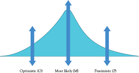
Figure 7.6 PERT distribution curve
Advantages and Disadvantages of PERT
The advantages and disadvantages of PERT are as follows.
Advantages
• Interdependencies and problem areas that may not be obvious by other scheduling methods become obvious quickly due to the kind of detailed planning required to create the PERT network.
• The PERT method usually shows the critical path in an organized diagram and well-defined manner, therefore helping the project manager and other stakeholders to make quick and quality decisions to the benefit of the project.
• It enables “what if” analysis to be carried out on projects, that is, the effect of changes in the schedule, which helps identify the risks associated with activities. The possibilities and the various level of uncertainties can then be studied from the project activities by analyzing the critical path properly, enabling the most suitable combination (minimum cost, economy, and best result) to be chosen for the project.
• It enables the determination of the probability of meeting specified deadlines by development of alternatives plans since statistical analysis such as standard deviations can be utilized with it.
• The activities and the events from the PERT networks can be analyzed independently as well as in combination to provide a picture of the likely completion of the project and the associated budget.
Disadvantages
• One of the greatest disadvantages of PERT is that it can be very complex, making it time- and labor-intensive to operate.
• Additionally, due to a large data requirement, PERT is an expensive technique to maintain and is therefore mostly used in large complex projects and not in day-to-day management of smaller projects.
• The activities for a project are identified based on available data, but finding data for new or nonrepetitive projects is often difficult, leading to the use of subjective, biased, or unreliable information, which could lead to inaccurate estimated time.
• Predictions are often used to develop the PERT time, which could lead to the overall project achieving budget loss if the predictions and the decisions are inaccurate.
• PERT also has the disadvantage that it may result in a lack of functional ownership in estimates and assumes unlimited resources. However, this is usually not the case.
• The PERT method is reliant on estimation of different times to complete activities; therefore, it is not useful when no reasonable estimates of time can be made.
Graphical Evaluation and Review Technique
The graphical evaluation and review technique (GERT) is similar to PERT, but, as pointed out by Nicholas (2020), it has the distinct advantages of allowing for looping, branching, and multiple project end results. For example, with PERT, it cannot be easily shown that if an activity is unsuccessful; it may have to be repeated several times and one of several different branches can only be selected to continue the project. However, this challenge is easily overcome using GERT.
PDM, PERT, and CPM are limited as tools in their capacity to model a project realistically because of the following limitations as highlighted by Nicholas (2020):
• All immediate predecessor activities must be completed before a given activity can be started.
• No activity can be repeated, and no looping back to predecessors is permitted.
• The duration time for an activity is restricted to the beta distribution for PERT and a single estimate (deterministic) for CPM.
• The critical path is always considered the longest path even though variances include the likelihood of other paths being longer.
• There is only one terminal event and the only way to reach it is by completing all activities in the project.
The GERT technique overcomes these limitations as it permits alternative time distribution and allows looping back so that previous activities can be repeated as previously mentioned. The major distinction of GERT is that it utilizes complex nodes. In PERT, a node is an event that represents the start or finish of an activity and cannot be realized until all its immediate predecessors have been realized. GERT utilizes probabilistic and branching nodes that specify both the number of activities leading to them that must be realized as well as the potential multiple branching paths that can emanate from them.
Table 7.1 presents a summary of the differences that exist between the GERT and the CPM/PERT techniques as asserted by Meredith, Shafer, and Mantel (2021).
An Appraisal of the Suitability of the Time Control Techniques
The previous sections have presented most of the prevalent/classical project time control techniques that can be used for projects.
It could be noted from the Table 7.2 that quite often the project time control techniques have their own strengths and weaknesses. Therefore, for project time control, there is no one-cap-fits-all technique. For example, traditionally, the time control of the duration of projects has been carried out most frequently by means of Gantt charts. The problem with the Gantt bar chart is that it may not be effective for project time control. Some of the reasons for this were indicated in the weaknesses. First, the bar chart—although well known, simple, cheap to use, and familiar as a means of communication—has the following disadvantages: planning and scheduling must be carried out at one and the same time as the bars are constructed; dependencies of one operation or activity on others are not shown; control is restricted to that of duration, and it is not easy to connect the physical quantities of work involved in each operation with specific period. Therefore, the time progress does not necessarily give an accurate indication of the actual physical progress of the work.
Table 7.1 Differences between GERT and PERT/CPM
| GERT | PERT/CPM |
1 | Branching from a node is probabilistic | Branching from a node is deterministic |
2 | Various possible probability | Only the beta distribution for time estimates |
3 | Flexibility in node realization | No flexibility in node realization |
4 | Looping back to earlier events is acceptable | Looping back is not allowed |
5 | Difficult to use as a control tool | Easy to use as a control tool |
6 | Arc may represent time, cost, reliability, etc. | Arc represents time only |
It was discussed that the category of planning and scheduling methods that overcomes many of the disadvantages of the bar chart is that of network analysis. As mentioned in this chapter, network analysis covers a range of techniques; the most popular ones are CPM, PERT, and PDM. Network analysis methods, when used for time control of projects, were shown as having many advantages such as providing a systematic approach to planning; enabling modeling to test various project delivery options before the start of work; making possible the true effect of changes to a project to be analyzed insofar as the changes affect other activities; and depicting clearly the interrelationships between the activities of the project. They reveal interdependencies of activities; they facilitate “what if” exercises; they identify the longest path or critical paths; they aid in scheduling risk analysis (Kerzner 2017).
However, despite this overwhelming list of advantages, network methods of project control have been criticized since their inception, for example, by Nicholas (2020) for the following reasons: they incorporate assumptions and yield results that sometimes are unrealistic or pose problems to their users; network methods assume that a project can be completely defined as a sequence of identifiable, independent activities with known precedence relationships. In many projects, however, the work cannot be always anticipated, and not all activities can be clearly defined. Rather, projects evolve as they progress; it is difficult to demarcate one activity from the next, and the point of separation is arbitrary. Although the PDM helps overcome this difficulty in demarcating activities, precedence relationships are not always fixed with the start of one activity sometimes contingent upon the outcome of an earlier one, which may have to be repeated. The GERT method deals somewhat with this problem. Despite these disadvantages of network scheduling methods, it is important to note that network methods, though not perfect, are still the most helpful for project scheduling and time control and getting the best schedule estimate possible.
Table 7.2 Trait summary of existing project cost and time control techniques