
In the previous chapter, we learned to use R to extract information from web pages. To understand how this works, we learned several languages such as HTML, CSS, and XPath. In fact, R has much more to offer than just a statistical computing environment. The R community provides tools for everything from data collection, to data manipulation, statistical modeling, visualization, and all the way to reporting and presentation.
In this chapter, we will learn about a number of packages that boost our productivity. We'll review several languages we learned throughout this book and get to know another one: markdown. We'll see how R and markdown can be combined to produce powerful dynamic documents. More specifically, we'll:
- Get to know markdown and R Markdown
- Embed tables, charts, diagrams and interactive plots
- Create interactive apps
The work of data analysts is more than putting data into models and drawing some conclusions. We usually need to go through a complete workflow from data collecting, to data cleaning, visualization, modeling, and finally writing a report or making a presentation.
In the previous chapters, we improved our productivity by learning the R programming language from different aspects. In this chapter, we will further boost our productivity by focusing on the final step: reporting and presentation. In the following sections, we'll learn a very simple language to write documents: markdown.
Throughout this book, we have already learned a bunch of languages. These languages are very different and may confuse beginners. But if you keep in mind their purposes, it won't be hard to use them together. Before learning markdown, we'll take a quick review of the languages we learned in the previous chapters.
The first is, of course, the R programming language. A programming language is designed for solving problems. R is specially designed and tailored for statistical computing and is empowered by the community to be capable of doing many other things; the example is shown as follows:
n <- 100
x <- rnorm(n)
y <- 2 * x + rnorm(n)
m <- lm(y ~ x)
coef(m)
In Chapter 12, Data Manipulation, we learned SQL to query relational databases. It is designed to be a programming language but is used to express relational database operations such as inserting or updating records and querying data:
SELECT name, price
FROM products
WHERE category = 'Food'
ORDER BY price desc
The R programming language is executed by the R interpreter and SQL is executed by a database engine. However, we also learned languages that are not designed for execution but to represent data. Perhaps the most commonly used data representation languages in programming world are JSON and XML:
[
  {
    "id": 1,
    "name": "Product-A",
    "price": 199.95
  },
  {
    "id": 2,
    "name": "Product-B",
    "price": 129.95
  }
]
The specification of JSON defines elements such as value (1, "text"), array ([]), and object ({}), and so on, while XML does not provide type support but allows the usage of attributes and nodes:
<?xml version="1.0"?>
<root>
  <product id="1">
    <name>Product-A<name>
    <price>$199.95</price>
  </product>
  <product id="2">
    <name>Product-B</name>
    <price>$129.95</price>
  </product>
</root>
In the previous chapter on web scraping, we learned the basics of HTML which is quite similar to XML. Most web pages are written in HTML due to its flexible representation of contents and layouts:
<!DOCTYPE html>
<html>
<head>
  <title>Simple page</title>
</head>
<body>
  <h1>Heading 1</h1>
  <p>This is a paragraph.</p>
</body>
</html>
In this chapter, we'll learn markdown, a lightweight markup language with a syntax designed for plain text formatting and which can be converted to many other document formats. After getting familiar with markdown, we'll go further with R Markdown, which is designed for dynamic documents and is actively supported by RStudio and the rest of the R community. The format is so simple that we can use any plain text editor to write markdown documents.
The following code block shows its syntax:
# Heading 1 This is a top level section. This paragraph contains both __bold__ text and _italic_ text. There are more than one syntax to represent **bold** text and *italic* text. ## Heading 2 This is a second level section. The following are some bullets. * Point 1 * Point 2 * Point 3 ### Heading 3 This is a third level section. Here are some numbered bullets. 1. hello 2. world Link: [click here](https://r-project.org) Image:  Image link: [](https://r-project.org)
The syntax is extremely simple: Some characters are devoted to representing different formats. In a plain text editor, we cannot preview the formats as it indicates. But when converted to a HTML document, the texts will be formatted according to the syntax.
The following screenshot shows the preview of a markdown document in Abricotine (http://abricotine.brrd.fr/), an open-source markdown editor with live preview:

There are also online markdown editors with fantastic features. One of my favorites is StackEdit (https://stackedit.io/). You can create a new blank document and copy the above markdown texts into the editor, and then the you can see the instant preview as an HTML page:

Markdown is widely used in online discussion. The largest open-source repository host, GitHub (https://github.com), supports markdown in writing issues as shown in the following screenshot:

Note that backticks (`) are used to create source code symbols and three-backticks (```X) are used to contain a code block written in language X. Code blocks are shown in fixed-width font which is better for presenting program code. Also, we can preview what we have written so far:

Another special symbol, $, is used to quote math formulas. Single dollar ($) indicates inline math whereas double dollars ($$) displays math (in a new line). The math formula should be written in LaTeX math syntax (https://en.wikibooks.org/wiki/LaTeX/Mathematics).
The following math equation is not that simple: $$x^2+y^2=z^2$$, where $x$,$y$, and $z$ are integers.
Not all markdown editors support the preview of math formulas. In StackEdit, the preceding markdown is previewed as follows:

In addition, many markdown renderers support the table syntax shown as follows:
| Sepal.Length| Sepal.Width| Petal.Length| Petal.Width|Species |
|------------:|-----------:|------------:|-----------:|:-------|
|          5.1|         3.5|          1.4|         0.2|setosa  |
|          4.9|         3.0|          1.4|         0.2|setosa  |
|          4.7|         3.2|          1.3|         0.2|setosa  |
|          4.6|         3.1|          1.5|         0.2|setosa  |
|          5.0|         3.6|          1.4|         0.2|setosa  |
|          5.4|         3.9|          1.7|         0.4|setosa  |
In StackEdit, the preceding text table is rendered as follows:

Markdown is easy to write and read, and has most necessary features for writing reports such as simple text formatting, embedding images, links, tables, quotes, math formula, and code blocks.
Although writing plain texts in markdown is easy, creating reports with many images and tables is not, especially when the images and tables are produced dynamically by code. R Markdown is the killer app that integrates R into markdown.
More specifically, the markdowns we showed earlier in this chapter are all static documents; that is, they were determined when we wrote them. However, R Markdown is a combination of R code and markdown texts. The output of R code can be text, table, images, and interactive widgets. It can be rendered as an HTML web page, a PDF document, and even a Word document. Visit http://rmarkdown.rstudio.com/formats.html to learn more about supported formats.
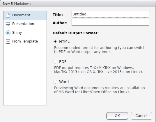
To create an R Markdown document, click the menu item, as shown in the following screenshot:

If you don't have rmarkdown and knitr installed, RStudio will install these necessary packages automatically. Then you can write a title and author and choose a default output format, as shown in the following screenshot:
Then a new R Markdown document will be created. The new document is not empty but a demo document that shows the basics of writing texts and embedding R code which produces images. In the template document, we can see some code chunks like:

The preceding chunk evaluates summary(cars) and will produce some text output:

The preceding chunk evaluates plot(pressure) and will produce an image. Note that we can specify options for each chunk in the form of {r [chunk_name], [options]} where [chunk_name] is optional and is used to name the produced image and [options] is optional and may specify whether the code should appear in the output document, the width and height of the produced graphics, and so on. To find more options, visit http://yihui.name/knitr/options/.
To render the document, just click on the Knit button:
When the document is properly saved to disk, RStudio will call functions to render the document into a web page. More specifically, the document is rendered in two steps:
- The
knitrmodule runs the code of each chunk and places the code and output according to the chunk options so thatRmdis fully rendered as a static markdown document. - The
pandocmodule renders the resulted markdown document as HTML, PDF, or DOCX according to theRmdoptions specified in file header.
As we are editing an R Markdown document in RStudio, we can choose which format to produce anytime and then it will automatically call the knitr module to render the document into markdown and then run the pandoc module with the proper arguments to produce a document in that format. This can also be done with code using functions provided by knitr and rmarkdown modules.
In the new document dialog, we can also choose presentation and create slides using R Markdown. Since writing documents and writing slides are similar, we won't go into detail on this topic.
Without R code chunks, R Markdown is no different from a plain markdown document. With code chunks, the output of code is embedded into the document so that the final content is dynamic. If a code chunk uses a random number generator without fixing the random seed, each time we knit the document we will get different results.
By default, the output of a code chunk is put directly beneath the code in fixed-width font starting with ## as if the code is run in the console. This form of output works but is not always satisfactory, especially when we want to present the data in more straightforward forms.
When writing a report, we often need to put tables within the contents. In an R Markdown document, we can directly evaluate a data.frame variable. Suppose we have the following data.frame:
toys <- data.frame(
  id = 1:3,
  name = c("Car", "Plane", "Motocycle"),
  price = c(15, 25, 14),
  share = c(0.3, 0.1, 0.2),
  stringsAsFactors = FALSE
)
To output the variable in plain text, we only need to type the variable name in a code chunk:
toys
##   id      name price share
## 1  1       Car    15   0.3
## 2  2     Plane    25   0.1
## 3  3 Motocycle    14   0.2
Note that HTML, PDF, and Word documents all support native tables. To produce a native table for the chosen format, we can use knitr::kable() to produce the markdown representation of the table just like the following:
| id|name      | price| share|
|--:|:---------|-----:|-----:|
|  1|Car       |    15|   0.3|
|  2|Plane     |    25|   0.1|
|  3|Motocycle |    14|   0.2|
When pandoc renders the resulted markdown document to other formats, it will produce a native table from the markdown representation:
knitr::kable(toys)
The table generated native table is shown as follows:
|
id |
name |
price |
share |
|
1 |
Car |
15 |
0.3 |
|
2 |
Plane |
25 |
0.1 |
|
3 |
Motocycle |
14 |
0.2 |
There are other packages that produce native tables but with enhanced features. For example, the xtable package not only supports converting data.frame to LaTeX, it also provides pre-defined templates to present the results of a number of statistical models.
xtable::xtable(lm(mpg ~ cyl + vs, data = mtcars))
When the preceding code is knitted with the results='asis' option, the linear model will be shown as the following table in the output PDF document:

The most well-known data software is perhaps Microsoft Excel. A very interesting feature of Excel is conditional formatting. To implement such features in R, I developed formattable package. To install, run install.packages("formattable"). It enables cell formatting in a data frame to exhibit more comparative information:
library(formattable)
formattable(toys,
  list(price = color_bar("lightpink"), share = percent))
The generated table is shown as follows:

Sometimes, the data has many rows, which makes embedding such a table into the document not a good idea. But JavaScript libraries such as DataTables (https://datatables.net/) make it easier to embed large data sets in a web page because it automatically performs paging and also supports search and filtering. Since an R Markdown document can be rendered into an HTML web page, it is natural to leverage the JavaScript package. An R package called DT (http://rstudio.github.io/DT/) ports DataTables to R data frames and we can easily put a large data set into a document to let the reader explore and inspect the data in detail:
library(DT)
datatable(mtcars)
The generated table is shown as follows:

The preceding packages, formattable and DT are two examples of a wide range of HTML widgets (http://www.htmlwidgets.org/). Many of them are adapted from popular JavaScript libraries since there are already a good number of high quality JavaScript libraries in the community.
Embedding charts is as easy as embedding tables as we demonstrated. If a code chunk produces a plot, knitr will save the image to a file with the name of the code chunk and write [name](image-file.png) below the code so that when pandoc renders the document the image will be found and inserted to the right place:
set.seed(123)
x <- rnorm(1000)
y <- 2 * x + rnorm(1000)
m <- lm(y ~ x)
plot(x, y, main = "Linear regression", col = "darkgray")
abline(coef(m))
The plot generated is shown as follows:

The default image size may not apply to all scenarios. We can specify chunk options fig.height and fig.width to alter the size of the image.
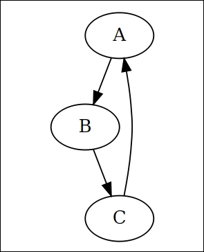
In addition to creating charts with basic graphics and packages like ggplot2, we can also create diagrams and graphs using DiagrammeR package. To install the package from CRAN, run install.packages("DiagrammeR").
This package uses Graphviz (https://en.wikipedia.org/wiki/Graphviz) to describe the relations and styling of a diagram. The following code produces a very simple directed graph:
library(DiagrammeR)
grViz("
digraph rmarkdown {
  A -> B;
  B -> C;
  C -> A;
}")
The generated graph is shown as follows:
DiagrammeR also provides a more programmable way to construct diagrams. It exports a set of functions to perform operations on a graph. Each function takes a graph and outputs a modified graph. Therefore it is easy to use pipeline to connect all operations to produce a graph in a streamline. For more details, visit the package website at http://rich-iannone.github.io/DiagrammeR.
Previously, we demonstrated both static tables (knitr::kable, xtable, and formattable) and interactive tables (DT). Similar things happen to plots too. We can not only place static images in the document as we did in the previous section, but also create dynamic and interactive plots in either the viewer or the output document.
In fact, there are more packages designed to produce interactive graphics than tables. Most of them take advantage of existing JavaScript libraries and make R data structures easier to work with them. In the following code, we introduce some of the most popular packages used to create interactive graphics.
The ggvis (http://ggvis.rstudio.com/) developed by RStudio uses Vega (https://vega.github.io/vega/) as its graphics backend:
library(ggvis)
mtcars %>%
  ggvis(~mpg, ~disp, opacity := 0.6) %>%
  layer_points(size := input_slider(1, 100, value = 50, label = "size")) %>%
  layer_smooths(span = input_slider(0.5, 1, value = 1, label = "span"))
The plot generated is shown as follows:
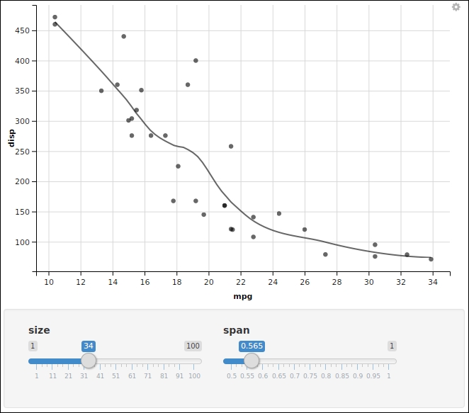
Note that its grammar is a bit like ggplot2. It best works with a pipeline operator.
Another package is called dygraphs (https://rstudio.github.io/dygraphs/) which uses the JavaScript library (http://dygraphs.com/) of the same name. This package specializes in plotting time series data with interactive capabilities.
In the following example, we use the temperature data of airports provided in the nycflights13 package. To plot the daily temperature time series of each airport present in the data, we need to summarize the data by computing the mean temperature on each day, reshape the long-format data to wide-format, and convert the results to an xts time series object with a date index and temperature columns corresponding to each airport:
library(dygraphs)
library(xts)
library(dplyr)
library(reshape2)
data(weather, package = "nycflights13")
temp <- weather %>%
  group_by(origin, year, month, day) %>%
  summarize(temp = mean(temp)) %>%
  ungroup() %>%
  mutate(date = as.Date(sprintf("%d-%02d-%02d",
    year, month, day))) %>%
  select(origin, date, temp) %>%
  dcast(date ~ origin, value.var = "temp")

temp_xts <- as.xts(temp[-1], order.by = temp[[1]])
head(temp_xts)
##                EWR     JFK      LGA
## 2013-01-01 38.4800 38.8713 39.23913
## 2013-01-02 28.8350 28.5425 28.72250
## 2013-01-03 29.4575 29.7725 29.70500
## 2013-01-04 33.4775 34.0325 35.26250
## 2013-01-05 36.7325 36.8975 37.73750
## 2013-01-06 37.9700 37.4525 39.70250
Then we supply temp_xts to dygraph() to create an interactive time series plot with a range selector and dynamic highlighting:
dygraph(temp_xts, main = "Airport Temperature") %>%
  dyRangeSelector() %>%
  dyHighlight(highlightCircleSize = 3,
    highlightSeriesBackgroundAlpha = 0.3,
    hideOnMouseOut = FALSE)
The plot generated is shown as follows:

If the code is run in R terminal, the web browser will launch and show a web page containing the plot. If the code is run in RStudio, the plot will show up in the Viewer pane. If the code is a chunk in R Markdown document, the plot will be embedded into the rendered document.
The main advantage of interactive graphics over static plots is that interactivity allows users to further examine and explore the data rather than forcing users to view it from a fixed perspective.
There are other remarkable packages of interactive graphics. For example, plotly (https://plot.ly/r/) and highcharter (http://jkunst.com/highcharter/) are nice packages to produce a wide range of interactive plots based on JavaScript backends.
In addition to the features we demonstrated in the previous sections, R Markdown can also be used to create presentation slides, journal articles, books and websites. Visit the official website at http://rmarkdown.rstudio.com to learn more.