
The S3 object system in R is a simple, loose, object-oriented system. Every basic object type has an S3 class name. For example, integer, numeric, character, logical, list,
data.frame, and so on are all S3 classes.
For example, the type of vec1 class is double, which means the internal type or storage mode of vec1 is double floating numbers. However, its S3 class is numeric:
vec1 <- c(1, 2, 3)
typeof(vec1)
## [1] "double"
class(vec1)
## [1] "numeric"
The type of data1 class is list, which means the internal type or storage mode of data1 is a list, but its S3 class is data.frame:
data1 <- data.frame(x = 1:3, y = rnorm(3))
typeof(data1)
## [1] "list"
class(data1)
## [1] "data.frame"
In the following sections, we'll explain the difference between the internal type of an object and its S3 class.
As we mentioned earlier in this chapter, a class can possess a number of methods that define its behavior, mostly with other objects. In the S3 system, we can create generic functions and implement them for different classes as methods. This is how the S3 method dispatch works to make the class of an object important.
There are many simple examples of the S3 generic function in R. Each of them is defined for a general purpose and allows different classes of objects to have their own implementation for that purpose. Let's first take a look at the head() and tail() functions. Their functionality is simple: head() gets the first n records of a data object, while tail() gets the last n records of a data object. It is different fromx[1:n] because it has different definitions of record for different classes of objects. For an atomic vector (numeric, character, and so on), the first n records just means the first n elements. However, for a data frame, the first n record means the first n rows rather than columns. Since a data frame is essentially a list, directly taking out the first n elements from a data frame is actually taking out the first n columns, which is not what head() is intended for.
First, let's type head and see what's inside the function:
head
## function (x, ...)
## UseMethod("head")
## <bytecode: 0x000000000f052e10>
## <environment: namespace:utils>
We find that there are no actual implementation details in this function. Instead, it calls UseMethod("head") to make head a so-called generic function to perform method dispatch, that is, it may behave in different ways for different classes.
Now, let's create two data objects of numeric class and data.frame class, respectively, and see how method dispatch works when we pass each object to the generic function head:
num_vec <- c(1, 2, 3, 4, 5)
data_frame <- data.frame(x = 1:5, y = rnorm(5))
For a numeric vector, head simply takes its first several elements.
head(num_vec, 3)
## [1] 1 2 3
However, for a data frame, head takes its first several rows rather than columns:
head(data_frame, 3)
##   x         y
## 1 1 0.8867848
## 2 2 0.1169713
## 3 3 0.3186301
Here, we can use a function to mimic the behavior of head. The following code is a simple implementation that takes the first n elements of any given object x:
simple_head <- function(x, n) {
  x[1:n]
}
For a numeric vector, it works in exactly the same way as head:
simple_head(num_vec, 3)
## [1] 1 2 3
However, for a data frame, it actually tries to take out the first n columns. Recall that the data frame is a list, and each column of the data frame is an element of the list. It may cause an error if n exceeds the number of columns of the data frame or, equivalently, the number of elements of the list:
simple_head(data_frame, 3)
## Error in `[.data.frame`(x, 1:n): undefined columns selected
To improve the implementation, we can check whether the input object x is a data frame before taking any measures:
simple_head2 <- function(x, n) {
  if (is.data.frame(x)) {
    x[1:n,]
  } else {
    x[1:n]
  }
}
Now, the behavior of simple_head2 is almost the same with head for atomic vectors and data frames:
simple_head2(num_vec, 3)
## [1] 1 2 3
simple_head2(data_frame, 3)
##   x         y
## 1 1 0.8867848
## 2 2 0.1169713
## 3 3 0.3186301
However, head offers more than this. To see the methods implemented for head, we can call methods(), which returns a character vector:
methods("head")
## [1] head.data.frame* head.default*    head.ftable*
## [4] head.function*   head.matrix      head.table*
## see '?methods' for accessing help and source code
It shows that there is already a bunch of built-in methods of head for a number of classes other than vectors and data frames. Note that the methods are all in the form of method.class. If we input a data.frame object, head will call head.data.frame internally. Similarly, if we input a table object, it will call head.table internally. What if we input a numeric vector? When no method is found that matches the class of the input object, it will turn to method.default, if defined. In this case, all atomic vectors are matched by head.default. The process through which a generic function finds the appropriate method for a certain input object is called method dispatch.
It looks like we can always check the class of the input object in a function to achieve the goal of method dispatch. However, it is easier to implement a method for another class to extend the functionality of a generic function because you don't have to modify the original generic function by adding specific class-checking conditions each time. We'll cover this later in this section.
S3 generic functions and methods are most useful in unifying the way we work with all kinds of models. For example, we can create a linear model and use generic functions to view the model from different perspectives:
lm1 <- lm(mpg ~ cyl + vs, data = mtcars)
In previous chapters, we mentioned that a linear model is essentially a list of data fields resulted from model fitting. That's why the type of lm1 is list, but its class is lm so that generic functions will choose methods for lm:
typeof(lm1)
## [1] "list"
class(lm1)
## [1] "lm"
The S3 method dispatch even happens without explicit calling of S3 generic functions. If we type lm1 and see what it is, the model object is printed:
lm1
##
## Call:
## lm(formula = mpg ~ cyl + vs, data = mtcars)
##
## Coefficients:
## (Intercept)          cyl           vs
##     39.6250      -3.0907      -0.9391
In fact, print is implicitly called:
print(lm1)
##
## Call:
## lm(formula = mpg ~ cyl + vs, data = mtcars)
##
## Coefficients:
## (Intercept)          cyl           vs
##     39.6250      -3.0907      -0.9391
We know that lm1 is essentially a list. Why does it not look like a list when it is printed? This is because print is a generic function, and it has a method for lm that prints the most important information of the linear model. We can get the actual method we call by getS3method("print", "lm"). In fact, print(lm1) goes to stats:::print.lm, which can be verified by checking whether they are identical:
identical(getS3method("print", "lm"), stats:::print.lm)
## [1] TRUE
Note that print.lm is defined in the stats package, but is not exported for public use, so we have to use ::: to access it. Generally, it is a bad idea to access internal objects in a package, because they may change in different releases and have no changes visible to the user. In most cases, we simply don't need to because generic functions such as print automatically choose the right method to call.
In R, print has methods implemented for many classes. The following code shows how many methods are implemented for different classes:
length(methods("print"))
## [1] 198
You can call methods("print") to view the whole list. In fact, if more packages are loaded, there will be more methods defined for classes in these packages.
While print shows a brief version of the model, summary shows detailed information. This function is also a generic function that has many methods for all kinds of model classes:
summary(lm1)
##
## Call:
## lm(formula = mpg ~ cyl + vs, data = mtcars)
##
## Residuals:
##    Min     1Q Median     3Q    Max
## -4.923 -1.953 -0.081  1.319  7.577
##
## Coefficients:
##             Estimate Std. Error t value Pr(>|t|)
## (Intercept)  39.6250     4.2246   9.380 2.77e-10 ***
## cyl          -3.0907     0.5581  -5.538 5.70e-06 ***
## vs           -0.9391     1.9775  -0.475    0.638
## ---
## Signif. codes:
## 0 '***' 0.001 '**' 0.01 '*' 0.05 '.' 0.1 ' ' 1
##
## Residual standard error: 3.248 on 29 degrees of freedom
## Multiple R-squared:  0.7283, Adjusted R-squared:  0.7096
## F-statistic: 38.87 on 2 and 29 DF,  p-value: 6.23e-09
The summary of a linear model provides not only what print shows but also some important statistics for the coefficients and the overall model. In fact, the output of summary is another object that can be accessed for the data it contains. In this case, it is a list of the summary.lm class, and it has its own method of print:
lm1summary <- summary(lm1)
typeof(lm1summary)
## [1] "list"
class(lm1summary)
## [1] "summary.lm"
To list what elements lm1summary contains, we can view the names on the list:
names(lm1summary)
## [1] "call"          "terms"         "residuals"
## [4] "coefficients"  "aliased"       "sigma"
## [7] "df"            "r.squared"     "adj.r.squared"
##[10] "fstatistic"    "cov.unscaled"
We can access each element in exactly the same way as we extract an element from a typical list. For example, to access the estimated coefficients of the linear model, we can use lm1$coefficients. Alternatively, we will use the following code to access the estimated coefficients:
coef(lm1)
## (Intercept)         cyl          vs
##  39.6250234  -3.0906748  -0.9390815
Here, coef is also a generic function that extracts the vector of coefficients from a model object. To access the detailed coefficient table in the model summary, we can use lm1summary$coefficients or, again, coef:
coef(lm1summary)
##               Estimate Std. Error    t value     Pr(>|t|)
## (Intercept) 39.6250234  4.2246061  9.3795782 2.765008e-10
## cyl         -3.0906748  0.5580883 -5.5379676 5.695238e-06
## vs          -0.9390815  1.9775199 -0.4748784 6.384306e-01
There are other useful model-related generic functions such as plot, predict, and so on. All these generic functions we mentioned are standard ways in R for users to interact with an estimated model. Different built-in models and those provided by third-party packages all try to implement these generic functions so that we don't need to remember different sets of functions to work with each model.
For example, we can use the plot function to the linear model with 2-by-2 partitions:
oldpar <- par(mfrow = c(2, 2))
plot(lm1)
par(oldpar)
This produces the following image with four parts:

We can see that we used plot function to a linear model, which will result in four diagnostic plots that show the features of the residuals, which can be helpful in getting an impression on whether the model fit is good or bad. Note that if we directly call the plot function to a lm in a console, the four plots are interactively done in turn. To avoid this, we call par() to divide the plot area into 2-by-2 subareas.
Most statistical models are useful because they can be used to predict with new data. To do this, we use predict. In this case, we can supply the linear model and the new data to predict, and it will find the right method to make predictions with new data:
predict(lm1, data.frame(cyl = c(6, 8), vs = c(1, 1)))
##        1        2
## 20.14189 13.96054
This function can be used both in sample and out of sample. If we supply new data to the model, it is out-of-sample prediction. If the data we supply is already in the sample, it is in-sample prediction. Here, we can create a scatter plot between actual values (mtcars$mpg) and fitted values to see how well the fitted linear model predicts:
plot(mtcars$mpg, fitted(lm1))
The plot generated is shown as follows:

Here, fitted is also a generic function, which, in this case, is equivalent to lm1$fitted.values, fitted values are also equal to the predicted values with the original dataset using predict(lm1, mtcars).
The difference between the actual values and fitted values of the response variable is called residuals. We can use another generic function residuals to access the numeric vector, or equivalently, use lm1$residuals. Here, we will make a density plot of the residuals:
plot(density(residuals(lm1)),
  main = "Density of lm1 residuals")
The plot generated is shown as follows:

In the preceding function call, all involved functions are generic functions. The residuals function extracts the residuals from lm1 and returns a numeric vector. The density function creates a list of class density to store the estimated data of density function of the residuals. Finally, plot turns to plot.density to create a density plot.
These generic functions work not only with lm, glm, and other built-in models, but also with models provided by other packages. For example, we use the rpart package to fit a regression tree model using the same data and the same formula in the previous example.
If you don't have the package installed, you need run the following code:
install.packages("rpart")
Now, the package is ready to attach. We call rpart in exactly the same way as lm:
library(rpart)
tree_model <- rpart(mpg ~ cyl + vs, data = mtcars)
We can do so because the package authors want the function call to be consistent with how we call built-in functions in R. The resulted object is a list of class rpart, which works in the same way with lm is a list of class rpart:
typeof(tree_model)
## [1] "list"
class(tree_model)
## [1] "rpart"
Like lm object, rpart also has a number of generic methods implemented. For example, we use the print function to print the model in its own way:
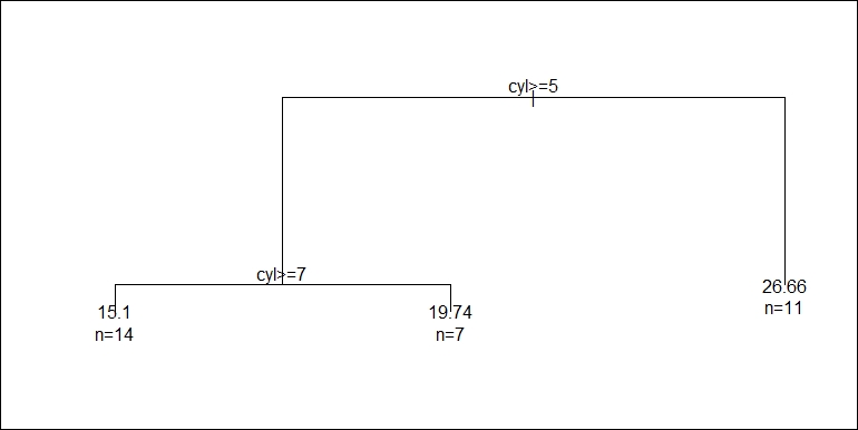
print(tree_model)
## n = 32
##
## node), split, n, deviance, yval
##       * denotes terminal node
##
## 1) root 32 1126.04700 20.09062
##   2) cyl >= 5 21  198.47240 16.64762
##     4) cyl >= 7 14   85.20000 15.10000 *
##     5) cyl < 7 7   12.67714 19.74286 *
##   3) cyl < 5 11  203.38550 26.66364 *
The output indicates that print has a method for rpart, which briefly shows what the regression tree looks like. In addition to print, summary gives more detailed information about the model fitting:
summary(tree_model)
## Call:
## rpart(formula = mpg ~ cyl + vs, data = mtcars)
##   n = 32
##
##           CP nsplit rel error    xerror       xstd
## 1 0.64312523      0 1.0000000 1.0844542 0.25608044
## 2 0.08933483      1 0.3568748 0.3858990 0.07230642
## 3 0.01000000      2 0.2675399 0.3875795 0.07204598
##
## Variable importance
## cyl  vs
##  65  35
##
## Node number 1: 32 observations,    complexity param=0.6431252
##   mean=20.09062, MSE=35.18897
##   left son=2 (21 obs) right son=3 (11 obs)
##   Primary splits:
##       cyl < 5   to the right, improve=0.6431252, (0 missing)
##       vs  < 0.5 to the left,  improve=0.4409477, (0 missing)
##   Surrogate splits:
##       vs < 0.5 to the left,  agree=0.844, adj=0.545, (0 split)
##
## Node number 2: 21 observations,    complexity param=0.08933483
##   mean=16.64762, MSE=9.451066
##   left son=4 (14 obs) right son=5 (7 obs)
##   Primary splits:
##       cyl < 7   to the right, improve=0.5068475, (0 missing)
##   Surrogate splits:
##       vs < 0.5 to the left,  agree=0.857, adj=0.571, (0 split)
##
## Node number 3: 11 observations
##   mean=26.66364, MSE=18.48959
##
## Node number 4: 14 observations
##   mean=15.1, MSE=6.085714
##
## Node number 5: 7 observations
##   mean=19.74286, MSE=1.81102
Likewise, plot and text also have methods for rpart to visualize it:
oldpar <- par(xpd = NA)
plot(tree_model)
text(tree_model, use.n = TRUE)
par(oldpar)
Then, we have the following tree graph:
We can use predict to make predictions with new data, just like what we did with the linear model in the previous examples:
predict(tree_model, data.frame(cyl = c(6, 8), vs = c(1, 1)))
##        1        2
## 19.74286 15.10000
Note that not all models implement methods for all the generic functions. For example, since the regression tree is not a simple parametric model, it does not implement a method for coef:
coef(tree_model)
## NULL
In the previous section, you learned how to use existing classes and methods to work with model objects. The S3 system, however, also allows us to create our own classes and generic functions.
Recall the example where we used conditional expressions to mimic the method dispatch of head. We mentioned that it works, but is often not the best practice. S3 generic functions are more flexible and easier to extend. To define a generic function, we usually create a function in which
UseMethod is called to trigger method dispatch. Then, we create method functions in the form of method.class for the classes we want the generic function to work with and usually a default method in the form of method.default to capture all other cases. Here is a simple rewriting of this example using generic function and methods. Here, we will create a new generic function, generic_head, with two arguments: the input object x and the number of records to take, n. The generic function only calls UseMethod("generic_head") to ask R for method dispatch according to the class of x:
generic_head <- function(x, n)
  UseMethod("generic_head")
For atomic vectors (numeric, character, logical, and so on), the first n elements should be taken. We can define generic_head.numeric, generic_head.character, and so on respectively, but in this case, it looks better to define a default method to capture all cases that are not matched by other generic_head.class methods:
generic_head.default <- function(x, n) {
  x[1:n]
}
Now, generic_head has only one method, which is equivalent to not using generic function at all:
generic_head(num_vec, 3)
## [1] 1 2 3
Since we haven't defined the method for class data.frame, supplying a data frame will fall back to generic_head.default, which causes an error due to the invalid access of an out-of-bound column index:
generic_head(data_frame, 3)
## Error in `[.data.frame`(x, 1:n): undefined columns selected
However, let's assume we define a method for data.frame:
generic_head.data.frame <- function(x, n) {
  x[1:n,]
}
The generic function works as it is supposed to:
generic_head(data_frame, 3)
##   x         y
## 1 1 0.8867848
## 2 2 0.1169713
## 3 3 0.3186301
You may notice that the methods we implemented earlier are not robust because we don't have the argument checked. For example, if n is greater than the number of elements of the input object, the function will behave differently and usually in an undesirable way. I'll leave it as an exercise for you to make the methods more robust and behave appropriately for corner cases.
Now, it is time to have some examples of defining new classes. Note that class(x) gets the class of x, while class(x) <- "some_class" sets the class of x to some_class.
Just like lm and rpart, list is probably the most widely used underlying data structure to create a new class. This is because a class represents a type of object that can store different kinds of data with different lengths and has some methods to interact with other objects.
In the following example, we will define a function called product that creates a list of the class product with a name, price, and inventory. We'll define its own print method and add more behaviors as we go ahead:
product <- function(name, price, inventory) {
  obj <- list(name = name,
    price = price,
    inventory = inventory)
  class(obj) <- "product"
  obj
}
Note that we created a list first, replaced its class with product, and finally returned the object. In fact, the class of an object is a character vector. An alternative way is to use structure():
product <- function(name, price, inventory) {
  structure(list(name = name,
    price = price,
    inventory = inventory),
    class = "product")
}
Now, we have a function that produced objects of the class product. In the following code, we will call product() and create an instance of this class:
laptop <- product("Laptop", 499, 300)
Like all previous objects, we can see its internal data structure and its S3 class for method dispatch:
typeof(laptop)
## [1] "list"
class(laptop)
## [1] "product"
Obviously, laptop is a list of class product as we created it. Since we haven't defined any methods for this class, its behavior is no different from an ordinary list object. If we type it, it will be printed as a list with its customized class attribute:
laptop
## $name
## [1] "Laptop"
##
## $price
## [1] 499
##
## $inventory
## [1] 300
##
## attr(,"class")
## [1] "product"
First, we can implement the print method for this class. Here, we want the class and the data fields in it to be printed in a compact style:
print.product <- function(x, ...) {
  cat("<product>
")
  cat("name:", x$name, "
")
  cat("price:", x$price, "
")
  cat("inventory:", x$inventory, "
")
  invisible(x)
}
It is a convention that the print method returns the input object itself for further use. If the printing is customized, then we often use invisible to suppress repeated printing of the same object that the function returns. You may try returning x directly and see what happens.
Then, we type the variable again. The print method will be dispatched to print.product since it is already defined:
laptop
## <product>
## name: Laptop
## price: 499
## inventory: 300
We can access the elements in laptop just like extracting elements from a list:
laptop$name
## [1] "Laptop"
laptop$price
## [1] 499
laptop$inventory
## [1] 300
If we create another instance and put the two instances into a list, print.product will still be called when the list is printed:
cellphone <- product("Phone", 249, 12000)
products <- list(laptop, cellphone)
products
## [[1]]
## <product>
## name: Laptop
## price: 499
## inventory: 300
##
## [[2]]
## <product>
## name: Phone
## price: 249
## inventory: 12000
This is because when products is printed as a list, it calls print on each of the elements, which also causes method dispatch.
Creating an S3 class is much simpler than most other programming languages that require formal definition of classes. It is important to have sufficient checking on the arguments to ensure that the created object is internally consistent with what the class represents.
For example, without proper checking, we can create a product with negative and non-integer inventory:
product("Basket", 150, -0.5)
## <product>
## name: Basket
## price: 150
## inventory: -0.5
To avoid this, we need to add some checking conditions in the object-generating function, product:
product <- function(name, price, inventory) {
  stopifnot(
    is.character(name), length(name) == 1,
    is.numeric(price), length(price) == 1,
    is.numeric(inventory), length(inventory) == 1,
price > 0, inventory >= 0)
  structure(list(name = name,
    price = as.numeric(price),
    inventory = as.integer(inventory)),
    class = "product")
}
The function is enhanced, in that name must be a single string, price must be a single positive number, and inventory must be a single non-negative number. With this function, we cannot create ridiculous products by mistake, and such errors can be found in an early stage:
product("Basket", 150, -0.5)
## Error: inventory >= 0 is not TRUE
In addition to defining new classes, we can also define new generic functions. In the following code, we will define a new generic function called value and implement a method for product by measuring the value of the inventory of the product:
value <- function(x, ...)
  UseMethod("value")

value.default <- function(x, ...) {
  stop("value is undefined")
}

value.product <- function(x, ...) {
  x$price * x$inventory
}
For other classes, it calls value.default and stops. Now, value can be used with all instances of product we created:
value(laptop)
## [1] 149700
value(cellphone)
## [1] 2988000
The generic function also works with apply family functions by performing method dispatch for each element in the input vector or list:
sapply(products, value)
## [1]  149700 2988000
One more question is once we create the object of a certain class, does that mean that we can no longer change it? No, we still can change it. In this case, we can modify an existing element of laptop:
laptop$price <- laptop$price * 0.85
We can also create a new element in laptop:
laptop$value <- laptop$price * laptop$inventory
Now, we can take a look at it, and the changes are effective:
laptop
## <product>
## name: Laptop
## price: 424.15
## inventory: 300
What's worse is that we can even remove an element by setting it to NULL. This is why the S3 system is considered to be loose. You can't make sure that the object of a certain type has a fixed set of data fields and methods.
In the previous section, we demonstrated an example of creating a new class from a list object. In fact, it is sometimes useful to create a new class of object from an atomic vector. In this section, I will show you a series of steps to create vectors with a percentage representation.
We first define a function, percent. This function simply checks whether the input is a numeric vector and alters its class to percent, which inherits from numeric:
percent <- function(x) {
  stopifnot(is.numeric(x))
  class(x) <- c("percent", "numeric")
  x
}
The inheritance here means that method dispatch first looks for methods of percent. If none is found, then it looks for methods of numeric. Therefore, the order of the class names matters. S3 inheritance will be covered in detail in the following section.
Now, we can create a percent vector from a numeric vector:
pct <- percent(c(0.1, 0.05, 0.25, 0.23))
pct
## [1] 0.10 0.05 0.25 0.23
## attr(,"class")
## [1] "percent" "numeric"
At the moment, there is no method implemented for percent. So, pct looks like an ordinary numeric vector with a customized class attribute. The purpose of this class is to show its values in percentage form, such as 25 percent instead of its original decimal representation.
To achieve this goal, we first implement as.character for the percent class by producing the correct string representation of the percentage form:
as.character.percent <- function(x, ...) {
  paste0(as.numeric(x) * 100, "%")
}
Now, we can get the desired string representation of a given percent vector:
as.character(pct)
## [1] "10%" "5%"  "25%" "23%"
Likewise, we need to implement format for percent by directly calling as.character:
format.percent <- function(x, ...) {
  as.character(x, ...)
}
Now, format has the same effect:
format(pct)
## [1] "10%" "5%"  "25%" "23%"
Now, we can implement print for percent by calling format.percent directly:
print.percent <- function(x, ...) {
  print(format.percent(x), quote = FALSE)
}
Note that we specify quote = FALSE when we print the formatted strings to make it look like numbers rather than strings. This is exactly the desired effect:
pct
## [1] 10% 5%  25% 23%
Note that arithmetic operators such as + and * automatically preserve the class of the output vector. As a result, the output vector is still printed in percentage form:
pct + 0.2
## [1] 30% 25% 45% 43%
pct * 0.5
## [1] 5%    2.5%  12.5% 11.5%
Unfortunately, other functions may not preserve the class of their input. For example, sum, mean, max, and min will drop the customized class and return a plain numeric vector instead:
sum(pct)
## [1] 0.63
mean(pct)
## [1] 0.1575
max(pct)
## [1] 0.25
min(pct)
## [1] 0.05
To make sure the percentage form is preserved when we perform these calculations, we need to implement these methods for the percent class:
sum.percent <- function(...) {
  percent(NextMethod("sum"))
}
mean.percent <- function(x, ...) {
  percent(NextMethod("mean"))
}
max.percent <- function(...) {
  percent(NextMethod("max"))
}
min.percent <- function(...) {
  percent(NextMethod("max"))
}
In the first method, NextMethod("sum") calls sum for numeric class, and the output numeric vector is wrapped with percent again. The same logic also applies to the implementation of the other three methods:
sum(pct)
## [1] 63%
mean(pct)
## [1] 15.75%
max(pct)
## [1] 25%
min(pct)
## [1] 5%
Now, these functions return values in percentage form, too. However, if we combine a percent vector with other numeric values, the percent class will be gone:
c(pct, 0.12)
## [1] 0.10 0.05 0.25 0.23 0.12
We can do the same thing to c:
c.percent <- function(x, ...) {
  percent(NextMethod("c"))
}
Now, combining percent vectors with numeric values result in percent vectors too:
c(pct, 0.12, -0.145)
## [1] 10%    5%     25%    23%    12%    -14.5%
However, from the other side, when we subset the percent vector or extract a value from it, the percent class will be dropped:
pct[1:3]
## [1] 0.10 0.05 0.25
pct[[2]]
## [1] 0.05
To fix this, we need to implement [ and [[ for percent in exactly the same way. You might be surprised to see a method called [.percent, but it will indeed match the percent class when we use these operators on a percent vector:
`[.percent` <- function(x, i) {
  percent(NextMethod("["))
}
`[[.percent` <- function(x, i) {
  percent(NextMethod("[["))
}
Now, both subsetting and extracting preserve the percent class:
pct[1:3]
## [1] 10% 5%  25%
pct[[2]]
## [1] 5%
With all these methods implemented, we can place a percent vector as a column of a data frame:
data.frame(id = 1:4, pct)
##   id pct
## 1  1 10%
## 2  2  5%
## 3  3 25%
## 4  4 23%
The percentage form is correctly preserved as a column in the data frame.
The S3 system is loose. You only need to create a function in the form of method.class to implement a method for a generic function. You only need to supply a character vector with multiple elements to indicate the inheritance relationship along the vector.
As we mentioned in the previous section, the class vector determines the order of matching classes in method dispatch. To demonstrate it, we will use a simple example in which we construct a number of classes with inheritance relationships.
Suppose we want to model some vehicles such as a car, bus, and airplane. These vehicles have something in common. They all have name, speed, and position, and they can move. To model them, we can define a base class called vehicle, which stores the common parts. We also define car, bus, and airplane that inherit from vehicle but have customized behaviors.
First, we will define a function to create the vehicle object, which is essentially an environment. We choose an environment over a list because we need its reference semantics, that is, we pass around the object, and modifying it will not cause a copy of the object. So, the object always refers to the same vehicle, no matter where it is passed around:
Vehicle <- function(class, name, speed) {
  obj <- new.env(parent = emptyenv())
  obj$name <- name
  obj$speed <- speed
  obj$position <- c(0, 0, 0)
  class(obj) <- c(class, "vehicle")
  obj
}
Note that class(obj) <- c(class, "vehicle") may look ambiguous because class is both a function argument and a basic function. In fact, class(obj) <- will look for the class<- function so that the usage does not cause ambiguity. The Vehicle function is a general creator of vehicle class objects with common data fields. The following function is specialized functions to create car, bus and airplane that inherit vehicle:
Car <- function(...) {
  Vehicle(class = "car", ...)
}
Bus <- function(...) {
  Vehicle(class = "bus", ...)
}
Airplane <- function(...) {
  Vehicle(class = "airplane", ...)
}
With the three preceding functions, we can create car, bus, and airplane objects. All inherit from the vehicle class. Now, we create an instance for each class:
car <- Car("Model-A", 80)
bus <- Bus("Medium-Bus", 45)
airplane <- Airplane("Big-Plane", 800)
Now, we will implement a common print method for vehicle:
print.vehicle <- function(x, ...) {
  cat(sprintf("<vehicle: %s>
", class(x)[[1]]))
  cat("name:", x$name, "
")
  cat("speed:", x$speed, "km/h
")
  cat("position:", paste(x$position, collapse = ", "))
}
Since no print.car, print.bus or print.airplane is defined, typing those variables will print them with print.vehicle:
car
## <vehicle: car>
## name: Model-A
## speed: 80 km/h
## position: 0, 0, 0
bus
## <vehicle: bus>
## name: Medium-Bus
## speed: 45 km/h
## position: 0, 0, 0
airplane
## <vehicle: airplane>
## name: Big-Plane
## speed: 800 km/h
## position: 0, 0, 0
A vehicle is a carrier designed to be driven and to move. Naturally, we define a generic function called move, which modifies the position of a vehicle to reflect a user-supplied movement in a three-dimensional space. Since different vehicles move in different ways with distinct limitations, we can further implement several move methods for the various classes of vehicle we just defined:
move <- function(vehicle, x, y, z) {
  UseMethod("move")
}
move.vehicle <- function(vehicle, movement) {
  if (length(movement) != 3) {
    stop("All three dimensions must be specified to move a vehicle")
  }
  vehicle$position <- vehicle$position + movement
  vehicle
}
Here, we will limit the movement that can happen to a car and a bus to two dimensions. Therefore, we will implement move.bus and move.car by checking the length of the movement vector, which is only allowed to be 2. If the movement is valid, then, we would force the third dimension of movement to be 0 and then call NextMethod("move") to call move.vehicle with vehicle and the latest value of movement:
move.bus <- move.car <- function(vehicle, movement) {
  if (length(movement) != 2) {
    stop("This vehicle only supports 2d movement")
  }
  movement <- c(movement, 0)
  NextMethod("move")
}
An airplane can move in either two or three dimensions. Therefore, move.airplane can be flexible to accept both. If the movement vector is two dimensional, then the movement on the third dimension is regarded as zero:
move.airplane <- function(vehicle, movement) {
  if (length(movement) == 2) {
    movement <- c(movement, 0)
  }
  NextMethod("move")
}
With move implemented for all three vehicles, we can test them with the three instances. First, let's see if the following expression goes into an error if we want the car to move with a three-dimensional vector:
move(car, c(1, 2, 3))
## Error in move.car(car, c(1, 2, 3)): This vehicle only supports 2d movement
The method dispatch of the preceding function call finds move.car and stops for the invalid movement. The following code is a two-dimensional movement, which is valid:
move(car, c(1, 2))
## <vehicle: car>
## name: Model-A
## speed: 80 km/h
## position: 1, 2, 0
Similarly, we can move the airplane in two dimensions:
move(airplane, c(1, 2))
## <vehicle: airplane>
## name: Big-Plane
## speed: 800 km/h
## position: 1, 2, 0
We can also move it in three dimensions:
move(airplane, c(20, 50, 80))
## <vehicle: airplane>
## name: Big-Plane
## speed: 800 km/h
## position: 21, 52, 80
Note that the position of airplane is accumulated because it is essentially an environment, so modifying position in move.vehicle does not cause a copy of it. Therefore, no matter where you pass it, there is only one instance of it. If you are not familiar with the reference semantics of environments, go through Chapter 8, Inside R.