Here, we will create a function called addn, which has one argument y. This function does not do the actual plus calculation but creates a child function that adds y to whatever number x supplied:

addn <- function(y) {
  function(x) {
    x + y
  }
} 

It may take extra efforts to realize that addn does not return a number like a typical function, but returns a closure: that is, a function defined in a function. The closure calculates x + y, where x refers to a local argument and y refers to an argument in its enclosing environment. In other words, addn() is no longer a calculator, but a calculator factory that manufactures calculators.

The factory function enables us to create specialized versions of calculators. For example, we can create two functions that add 1 and 2 to a numeric vector, respectively:

add1 <- addn(1)
add2 <- addn(2) 

The two functions work as if the second argument of add(x, y) was fixed. The following code validates the calculators made by addn():

add1(10)
## [1] 11
add2(10)
## [1] 12 

Take add1 as an example. The add1 <- addn(1) code evaluates addn(1), which results in a function assigned to add1:

add1
## function(x) {
## x + y
## }
## <environment: 0x00000000139b0e58> 

When we print add1, it is a bit different because the environment of add1 is also attached. The environment of a function will be printed if it is not the current environment-in this case, the global environment. In the environment of add1, y is specified in addn(1), which can be verified by running the following code:

environment(add1)$y
## [1] 1 

We can call environment() with add1 to access its enclosing environment, which captures y. That's exactly how closure works. We can do the same thing to add2 and see the value of y we specified with addn(2):

environment(add2)$y
## [1] 2 

Closures are useful to make specialized functions. For example, due to the flexibility of the production of graphics, plot functions often provide a large number of arguments. If we frequently use only a particular subset of all arguments, we can make specialized versions that make the code easier to write and read.

The following color_line function is a version of plot specialized in color picking, but with plot type and line type being fixed. It is comparable to a factory that makes pens of all colors:

color_line<- function(col) {
  function(...) {
    plot(..., type = "l", lty = 1, col = col)
  }
} 

If we want a red pen, we call color_line and get a specialized function that draws red lines. The resulted function is also open to other arguments such as title and font:

red_line<- color_line("red")
red_line(rnorm(30), main = "Red line plot") 

This function produces the following line plot:

The preceding code looks more readable than the original version that does not employ such a specialized function:

plot(rnorm(30), type = "l", lty = 1, col = "red",
  main = "Red line plot") 

Closures are useful when we work with an algorithm with some given data. Optimization, for example, is a problem to find a set of parameters that maximizes or minimizes a pre-defined objective function subject to certain constraints and data. In statistics, many parameter estimation problems are, in essence, optimization problems. One good example that demonstrates the use of closures is MLE (maximum likelihood estimation). When we estimate the parameters of a statistical model with data, we often use the method of maximal likelihood estimation (MLE, see https://en.wikipedia.org/wiki/Maximum_likelihood). The idea behind MLE is simple: the estimated values of parameters should make the observed data the most probable, given the model.

To perform MLE, we need a function that measures how probable it is to observe a given set of data under a specific model. Then, we apply optimization techniques to find out the values of parameters that maximizes the probability.

For example, we know that a set of observed data is generated by normal distribution, but the problem is, we don't know the parameters: mean and standard deviation. Then, we can use MLE to estimate them, given the observed data.

First, we know that the probability density function of a normal distribution with mean µ₀ and standard deviation Ïƒ₀ is:

Therefore, the likelihood function given the observed data x is:

To make the optimization easier, we will take a natural log and negate on both sides and get the negative log-likelihood function:

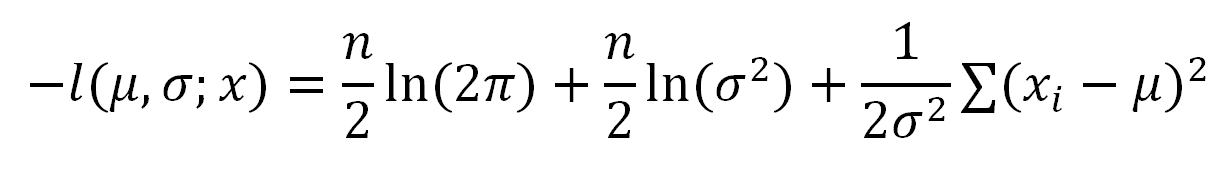
The negative log-likelihood function has the same monotonicity as the original function. The optimization solution of this function is the same as the original function but can be much easier to solve. That's why we use this function in the estimation.

The following nloglik R function returns a closure of the two parameters of normal distribution given the observed data x:

nloglik<- function(x) {
  n <- length(x)
  function(mean, sd) {
    log(2 * pi) * n / 2 + log(sd ^ 2) * n / 2 + sum((x - mean) ^ 2) / (2 * sd ^ 2)
  }
} 

In this way, for any given set of observations, we call nloglike to get a negative log-likelihood function with respect to mean and standard deviation. It tells us how unlikely it is for us to observe the given data x assuming that the true model takes the values of mean and sd we specify.

For example, we use rnorm() to generate 10,000 random numbers that are normally distributed with mean 1 and standard deviation 2. Therefore, mean = 1 and sd = 2 are the true values of the distribution parameters:

data <- rnorm(10000, 1, 2) 

Then, we turn to the mle() function in the stats4 package. This function implements a number of numeric methods to find the minimum value of a given negative log-likelihood function with certain parameters. It takes a starting point of the numeric search, and a lower bound and a upper bound of the solution:

fit <- stats4::mle(nloglik(data),
  start = list(mean = 0, sd = 1), method = "L-BFGS-B",
  lower =c(-5, 0.01), upper = c(5, 10)) 

After some iterations, it finds an MLE solution and returns an S4 object, which includes the related data of the solution. To see how close the estimates are to the true value, we will extract the coef slot from the object:

fit@coef
## mean sd
## 1.007548 1.990121 

It is obvious that the estimates are very close to the true values. Relatively speaking, both estimates have an error lower than 1 percent, as can be verified here:

(fit@coef - c(1, 2)) / c(1, 2)
## mean sd
##  0.007547752 -0.004939595 

The following function is a composition of the histogram of data and the density functions of the normal distribution with both true parameters (red curve) and estimated parameters (blue curve):

hist(data, freq =FALSE, ylim =c(0, 0.25))
curve(dnorm(x, 1, 2), add =TRUE, col =rgb(1, 0, 0, 0.5), lwd =6)
curve(dnorm(x, fit@coef[["mean"]], fit@coef[["sd"]]),
    add =TRUE, col ="blue", lwd =2) 

This produces the following histogram, plus a fitted normal density curve:

We can see that the density function produced by the estimated parameters is very close to the true model.

The first question is: if we assign an existing function to another variable, will it affect the enclosing environment of the function? If this is so, then the search paths of symbols that are not locally defined will be different.

The following code demonstrates why the enclosing environment of a function is not changed when it is assigned to another symbol. We define a simple function f1 that prints the executing environment, the enclosing environment, and the calling environment when it is called. Then, we define f2 that also prints the three environments, but in addition, it assigns the function of f1 to a local variable p and call p inside f2.

If p <- f1 defines the function locally, the enclosing environment of p will be the executing environment of f2. Otherwise, the enclosing environment will remain the global environment in which f1 is defined:

f1 <- function() {
  cat("[f1] executing in ")
  print(environment())
  cat("[f1] enclosed by ")
  print(parent.env(environment()))
  cat("[f1] calling from ")
  print(parent.frame())
}
f2 <- function() {
  cat("[f2] executing in ")
  print(environment())
  cat("[f2] enclosed by ")
  print(parent.env(environment()))
  cat("[f2] calling from ")
  print(parent.frame())
  p <- f1
  p()
}
f1()
## [f1] executing in <environment: 0x000000001435d700>
## [f1] enclosed by <environment: R_GlobalEnv>
## [f1] calling from <environment: R_GlobalEnv>
f2()
## [f2] executing in <environment: 0x0000000014eb2200>
## [f2] enclosed by <environment: R_GlobalEnv>
## [f2] calling from <environment: R_GlobalEnv>
## [f1] executing in <environment: 0x0000000014eaedf0>
## [f1] enclosed by <environment: R_GlobalEnv>
## [f1] calling from <environment: 0x0000000014eb2200> 

We called the two functions in turn and found that p is called from the executing environment of f2, but the enclosing environment is unchanged. In other words, the search path of p and f1 are exactly the same. In fact, p <- f1 assigns exactly the same function f1 represents to p, and then, they both point to the same function.

Functions in R are not as special as they are in other programming languages. Everything is an object. Functions are objects too and can be referred to by variables.

Suppose we have a function like this:

f1 <- function(x, y) {
  if (x > y) {
    x + y
  } else {
    x - y
  }
} 

In the preceding function, two conditional branches lead to different expressions that may result in different values. To achieve the same goal, we can also let the conditional branches result in different functions, store the result in a variable, and, finally, call the function the variable represents to get the result:

f2 <- function(x, y) {
  op <- if (x > y) `+` else `-`
  op(x, y)
} 

Note that in R, everything we do is done by a function. The most basic operators + and - are functions too. They can be assigned to the variable op, and we can call op if it is indeed a function.

The previous examples demonstrate that we can easily pass functions around just like everything else, including passing functions in arguments.

In the following example, we will define two functions called add and product, respectively:

add <- function(x, y, z) {
  x + y + z
}
product <- function(x, y, z) {
  x * y * z
} 

Then, we will define another function, combine, that tries to combine x, y, and z in some way specified by the argument f. Here,f is assumed to be a function that takes three arguments as we call it. In this way, combine is more flexible. It is not limited to a particular way of combining the inputs, but allows the user to specify:

combine <- function(f, x, y, z) {
  f(x, y, z)
} 

We can pass add and product, we just defined in turn, to see if it works:

combine(add, 3, 4, 5)
## [1] 12
combine(product, 3, 4, 5)
## [1] 60 

It is natural that when we call combine(add, 3, 4, 5), the function body has f = add and f(x, y, z), which result in add(x, y, z). The same logic also applies to calling combine with product. Since combine accepts a function in its first argument, it is indeed a higher-order function.

Another reason we need higher-order functions is that the code is easier to read and write at a higher level of abstraction. In many cases, using higher-order functions make the code shorter yet more expressive. For example, for-loop is an ordinary flow-control device that iterates along a vector or list.

Suppose we need to apply a function named f to each element of vector x. If the function itself is vectorized, it is better to call f(x) directly. However, not every function supports vectorized operations, nor does every function need to be vectorized. If we want to do so, a for-loop,like the following one, solves the problem:

result<-list()
for (i in seq_along(x)) {
    result[[i]] <-f(x[[i]])
}
result 

In the previous loop, seq_along(x) produces a sequence from 1 to the length of x, which is equivalent to 1:length(x). The code looks simple and easy to implement, but if we use it all the time, the drawback becomes significant.

Suppose the operation in each iteration gets more complicated: it would be hard to read. If you think about it, you will find that the code tells R how to finish the task instead of what the task is about. When you take a look at very long, sometimes nested loops, you would have a hard time to figure out what it is actually doing.

Instead, we can apply a function (f) to each element of a vector or list (x) by calling lapply, which we introduced in the previous chapters:

lapply(x, f) 

In fact, lapply is essentially the same as the following code, although it is implemented in C:

lapply <- function(x, f, ...) {
  result <- list()
  for (i in seq_along(x)) {
      result[[i]] <-f(x[i], ...)
  }
} 

This function is a higher-order function, because it works at a higher level of abstraction. Although it still uses a for-loop inside, it separates the work into two levels of abstraction so that each level looks simple.

In fact, lapply also supports extending f with additional arguments. For example, + has two arguments, as shown in the following code:

lapply(1:3, `+`, 3)
## [[1]]
## [1] 4
##
## [[2]]
## [1] 5
##
## [[3]]
## [1] 6 

The preceding lines of code are equivalent to:

list(1 +3, 2 +3, 3 +3) 

The preceding line of code is also equivalent to the case where we use a closure to produce the x+3 function:

lapply(1:3, addn(3))
## [[1]]
## [1] 4
##
## [[2]]
## [1] 5
##
## [[3]]
## [1] 6 

As we mentioned in the previous chapters, lapply only returns a list. If we want a vector instead, we should use sapply in the interactive mode:

sapply(1:3, addn(3))
## [1] 4 5 6 

Alternatively, we should use vapply in the programming code with type checking:

vapply(1:3, addn(3), numeric(1))
## [1] 4 5 6 

In addition to these functions, R also offers several other apply-family functions, as we mentioned in the previous chapters, as well as Filter, Map, Reduce, Find, Position, and Negate. For more details, refer to ?Filter in the documentation.

Moreover, the use of higher-order functions not only makes the code easier to read and more expressive, but these functions also separate the implementation of each level of abstraction so that they are independent from each other. It is much easier to improve simpler components than a whole bundle of logic coupled together.

For example, we can use apply-family functions to perform vector mapping, given a function. If each iteration is independent from the others, we can parallelize the mapping using multiple CPU cores so that more tasks can be done simultaneously. However, if we didn't use higher-order functions at the first place but a for-loop instead, it would take a while to convert it to parallel code.

For example, let's assume we use a for-loop to get the results. In each iteration, we perform a heavy computing task. Even if we find each iteration independently from the others, it is not always straightforward to convert it to parallel code:

result <- list()
for (i in seq_along(x)) {
  # heavy computing task
  result[[i]] <- f(x[[i]])
}
result 

However, if we use the higher-order function lapply(), things will be much easier:

result <- lapply(x, f) 

It would just take one small change to transform the code into a parallel version. Using parallel::mclapply(), we can apply f to each element of x with multiple cores:

result <- parallel::mclapply(x, f) 

Unfortunately, mclapply() does not support Windows. More code is needed to perform parallel apply functions in Windows. We will cover this topic in the chapter on high-performance computing.