I'm going to start by doing this the hard way. NumPy does have a method to just compute the covariance for you, and we'll talk about that later, but for now I want to show that you can actually do this from first principles:

%matplotlib inline 
 
import numpy as np 
from pylab import * 
 
def de_mean(x): 
    xmean = mean(x) 
    return [xi - xmean for xi in x] 
 
def covariance(x, y): 
    n = len(x) 
    return dot(de_mean(x), de_mean(y)) / (n-1) 

Covariance, again, is defined as the dot product, which is a measure of the angle between two vectors, of a vector of the deviations from the mean for a given set of data and the deviations from the mean for another given set of data for the same data's data points. We then divide that by n - 1 in this case, because we're actually dealing with a sample.

So de_mean(), our deviation from the mean function is taking in a set of data, x, actually a list, and it's computing the mean of that set of data. The return line contains a little bit of Python trickery for you. The syntax is saying, I'm going to create a new list, and go through every element in x, call it xi, and then return the difference between xi and the mean, xmean, for that entire dataset. This function returns a new list of data that represents the deviations from the mean for each data point.

My covariance() function will do that for both sets of data coming in, divided by the number of data points minus 1. Remember that thing about sample versus population in the previous chapter? Well, that's coming into play here. Then we can just use those functions and see what happens.

To expand this example, I'm going to fabricate some data that is going to try to find a relationship between page speeds, that, is how quickly a page renders on a website, and how much people spend. For example, at Amazon we were very concerned about the relationship between how quickly pages render and how much money people spend after that experience. We wanted to know if there is an actual relationship between how fast the website is and how much money people actually spend on the website. This is one way you might go about figuring that out. Let's just generate some normally distributed random data for both page speeds and purchase amounts, and since it's random, there's not going to be a real correlation between them.

pageSpeeds = np.random.normal(3.0, 1.0, 1000) 
purchaseAmount = np.random.normal(50.0, 10.0, 1000) 
 
scatter(pageSpeeds, purchaseAmount) 
 
covariance (pageSpeeds, purchaseAmount) 

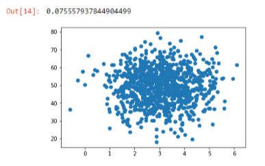
So just as a sanity check here we'll start off by scatter plotting this stuff:

You'll see that it tends to cluster around the middle because of the normal distribution on each attribute, but there's no real relationship between the two. For any given page speed is a wide variety of amount spent, and for any given amount spent there's a wide variety of page speeds, so no real correlation there except for ones that are coming out the randomness or through the nature of the normal distribution. Sure enough, if we compute the covariance in these two sets of attributes, we end up with a very small value, -0.07. So that's a very small covariance value, close to zero. That implies there's no real relationship between these two things.

Now let's make life a little bit more interesting. Let's actually make the purchase amount a real function of page speed.

purchaseAmount = np.random.normal(50.0, 10.0, 1000) / pageSpeeds 
 
scatter(pageSpeeds, purchaseAmount) 
 
covariance (pageSpeeds, purchaseAmount) 

Here, we are keeping things a little bit random, but we are creating a real relationship between these two sets of values. For a given user, there's a real relationship between the page speeds they encounter and the amount that they spend. If we plot that out, we can see the following output:

You can see that there's actually this little curve where things tend to be tightly aligned. Things get a little bit wonky near the bottom, just because of how random things work out. If we compute the covariance, we end up with a much larger value, -8, and it's the magnitude of that number that matters. The sign, positive or negative, just implies a positive or negative correlation, but that value of 8 says that's a much higher value than zero. So there's something going on there, but again it's hard to interpret what 8 actually means.

That's where the correlation comes in, where we normalize everything by the standard deviations as shown in the following code:

def correlation(x, y): 
stddevx = x.std() 
stddevy = y.std() 
return covariance(x,y) / stddevx / stddevy  #In real life you'd check for divide by zero here 
 
correlation(pageSpeeds, purchaseAmount) 

Again, doing that from first principles, we can take the correlation between two sets of attributes, compute the standard deviation of each, then compute the covariance between these two things, and divide by the standard deviations of each dataset. That gives us the correlation value, which is normalized to -1 to 1. We end up with a value of -0.4, which tells us there is some correlation between these two things in the negative direction:

It's not a perfect line, that would be -1, but there's something interesting going on there.