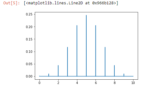
We can also visualize probability mass functions. This is called the binomial probability mass function. Again, we are going to use the same syntax as before, as shown in the following code:
from scipy.stats import expon
import matplotlib.pyplot as plt

x = np.arange(0, 10, 0.001)
plt.plot(x, expon.pdf(x))
So instead of expon or norm, we just use binom. A reminder: The probability mass function deals with discrete data. We have been all along, really, it's just how you think about it.
Coming back to our code, we're creating some discrete x values between 0 and 10 at a spacing of 0.01, and we're saying I want to plot a binomial probability mass function using that data. With the binom.pmf function, I can actually specify the shape of that data using two shape parameters, n and p. In this case, they're 10 and 0.5 respectively. output is shown on the following graph:

If you want to go and play around with different values to see what effects it has, that's a good way to get an intuitive sense of how those shape parameters work on the probability mass function.
