The main idea of boosting is that the elementary algorithms are not built independently. We build every sequential algorithm so that it corrects the mistakes of the previous ones and therefore improves the quality of the whole ensemble. The first successful version of boosting was AdaBoost (Adaptive Boosting). It is now rarely used since gradient boosting has supplanted it.

Suppose that we have a set of pairs, where each pair consists of attribute x and target variable y, . On this set, we restore the dependence of the form . We restore it by the approximation . To select the best approximation solution, we use a specific loss function of the form , which we should optimize as follows:

We also can rewrite the expression in terms of mathematical expectations, since the amount of data available for learning is limited, as follows:

Our approximation is inaccurate. However, the idea behind boosting is that such an approximation can be improved by adding to the model with the result of another model that corrects its errors, as illustrated here:

The following equation shows the ideal error correction model:

We can rewrite this formula in the following form, which is more suitable for the corrective model:

Based on the preceding assumptions listed, the goal of boosting is to approximate to make its results correspond as closely as possible to the residuals . Such an operation is performed sequentially—that is, improves the results of the
previous  function.

A further generalization of this approach allows us to consider the residuals as a negative gradient of the loss function, specifically of the form . In other words, gradient boosting is a method of GD with the loss function and its gradient replacement.

Now, knowing the expression of the loss function gradient, we can calculate its values ​​on our data. Therefore, we can train models so that our predictions are better correlated with this gradient (with a minus sign). Therefore, we will solve the regression problem, trying to correct the predictions for these residuals. For classification, regression, and ranking, we always minimize the squared difference between the residuals and our predictions.

In the gradient boosting method, an approximation of the function of the following form is used:

This is the sum of  functions of the  class; they are collectively called weak models (algorithms). Such an approximation is carried out sequentially, starting from the initial approximation, which is a certain constant, as follows:

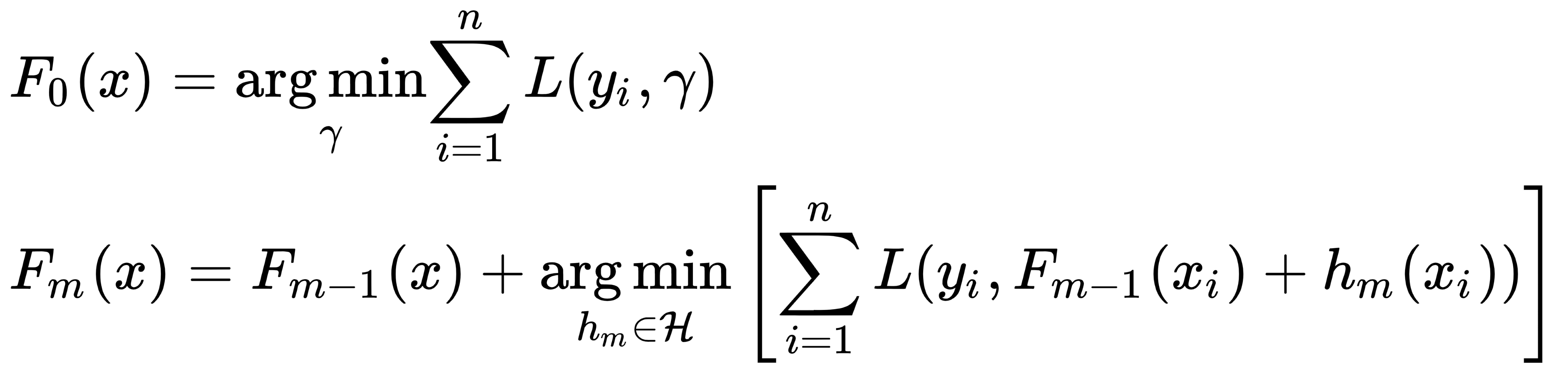
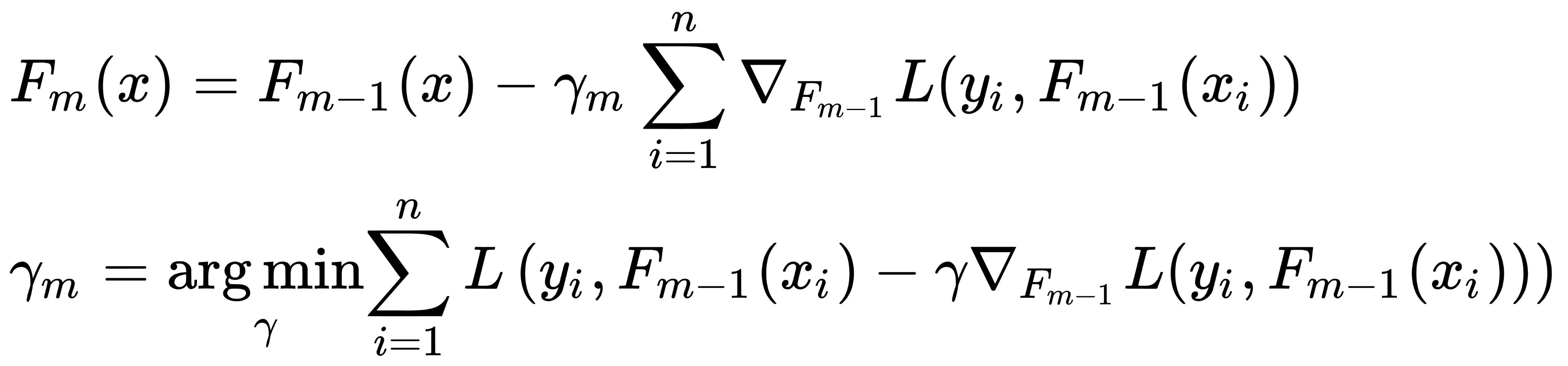
Unfortunately, the choice of the  optimal function at each step for an arbitrary loss function is extremely difficult, so a more straightforward approach is used. The idea is to use the GD method, by using differentiable  functions, and a differentiable loss function, as illustrated here:

The boosting algorithm is then formed as follows:

1. Initialize the model with constant values, like this:

2. Repeat the specified number of iterations and do the following:

• Calculate the pseudo-residuals, as follows:

Here, n is the number of training samples, m is the iteration number, and L is the loss function.

• Train the elementary algorithm (regression model)  on pseudo-residuals with data of the form .
• Calculate the coefficient by solving a one-dimensional optimization problem of the form, as follows:

• Update the model, as follows:

The inputs to this algorithm are as follows:

• The  dataset
• The number of M iterations
• The L( y, f ) loss function with an analytically written gradient (such a form of gradient allows us to reduce the number of numerical calculations)
• The choice of the family of functions of the h (x) elementary algorithms, with the procedure of their training and hyperparameters

The constant for the initial approximation, as well as the  optimal coefficient, can be found by a binary search, or by another line search algorithm relative to the initial loss function (rather than the gradient).

Examples of loss functions for regression are as follows:

•  : An L₂ loss, also called Gaussian loss. This formula is the classic conditional mean and the most common and simple option. If there are no additional information or model sustainability requirements, it should be used.
•  : An L₁ loss, also called Laplacian loss. This formula, at first glance, is not very differentiable and determines the conditional median. The median, as we know, is more resistant to outliers. Therefore, in some problems, this loss function is preferable since it does not penalize large deviations as much as a quadratic function.
•  : An L_q loss, also called Quantile loss. If we don't want a conditional median but do want a conditional 75 % quantile, we would use this option with . This function is asymmetric and penalizes more observations that turn out to be on the side of the quantile we need.

Examples of loss functions for classification are as follows:

• : This is logistic loss, also known as Bernoulli loss. An interesting property with this loss function is that we penalize even correctly predicted class labels. By optimizing this loss function, we can continue to distance classes and improve the classifier even if all observations are correctly predicted. This function is the most standard and frequently used loss function in a binary classification task.
• : This is AdaBoost loss. It so happens that the classic AdaBoost algorithm that uses this loss function (different loss functions can also be used in the AdaBoost algorithm) is equivalent to gradient boosting. Conceptually, this loss function is very similar to logistic loss, but it has a stronger exponential penalty for classification errors and is used less frequently.

The idea of bagging is that it can be used with a gradient boosting approach too, which is known as stochastic gradient boosting. In this way, a new algorithm is trained on a sub-sample of the training set. This approach can help us to improve the quality of the ensemble and reduces the time it takes to build elementary algorithms (whereby each is trained on a reduced number of training samples).

Although boosting itself is an ensemble, other ensemble schemes can be applied to it—for example, by averaging several boosting methods. Even if we average boosts with the same parameters, they will differ due to the stochastic nature of the implementation. This randomness comes from the choice of random sub-datasets at each step or selecting different features when we are building decision trees (if they are chosen as elementary algorithms).

Currently, the base gradient boosting machine (GBM) has many extensions for different statistical tasks. These are as follows:

• GLMBoost and GAMBoost as an enhancement of the existing generalized additive model (GAM)
• CoxBoost for survival curves
• RankBoost and LambdaMART for ranking

Secondly, there are many implementations of the same GBM under different names and different platforms, such as these:

• Stochastic GBM
• Gradient Boosted Decision Trees (GBDT)
• Gradient Boosted Regression Trees (GBRT)
• Multiple Additive Regression Trees (MART)
• Generalized Boosting Machines (GBM)

Furthermore, boosting can be applied and used over a long period of time in the ranking tasks undertaken by search engines. The task is written based on a loss function, which is penalized for errors in the order of search results; therefore, it became convenient to insert it into a GBM.