The first appearance of artificial neural networks can be traced to the article A logical calculus of the ideas immanent in nervous activity, which was published in 1943 by Warren McCallock and Walter Pitts. They proposed an early model of an artificial neuron. Donald Hebb, in his 1949 book The Organization of Behavior, described the basic principles of neuron training. These ideas were developed several years later by the American neurophysiologist Frank Rosenblatt. Rosenblatt invented the perceptron in 1957 as a mathematical model of the human brain's information perception. The concept was first implemented on a Mark-1 electronic machine in 1960.

Rosenblatt posited and proved the Perceptron Convergence Theorem (with the help of Blok, Joseph, Kesten, and other researchers who worked with him). It showed that an elementary perceptron, trained through error correction, regardless of the initial state of the weight coefficients and the sequence stimuli, always leads to a solution in a finite amount of time. Rosenblatt also presented evidence of some related theorems, which shows what conditions should correspond to the architecture of artificial neural networks and how they're trained. Rosenblatt also showed that the architecture of the perceptron is sufficient to obtain a solution to any conceivable classification task.

This means that the perceptron is a universal system. Rosenblatt himself identified two fundamental limitations of three-layer perceptrons (consisting of one S-layer, one A-layer, and R-layer): they lack the ability to generalize their characteristics in the presence of new stimuli or new situations, and the fact that they can't deal with complex situations, thus dividing them into simpler tasks.

Against the backdrop of the growing popularity of neural networks in 1969, a book by Marvin Minsky and Seymour Papert was published that showed the fundamental limitations of perceptrons. They showed that perceptrons are fundamentally incapable of performing many important functions. Moreover, at that time, the theory of parallel computing was poorly developed, and the perceptron was entirely consistent with the principles of this theory. In general, Minsky showed the advantage of sequential computing over parallel computing in certain classes of problems related to invariant representation. He also demonstrated that perceptrons do not have a functional advantage over analytical methods (for example, statistical methods) when solving problems related to forecasting. Some tasks that, in principle, can be solved by a perceptron require a very long time or a large amount of memory to solve them. These discoveries led to reorienting artificial intelligence researchers to the area of symbolic computing, which is the opposite of neural networks. Also, due to the complexity of mathematically studying perceptrons and there being a lack of generally accepted terminology, various inaccuracies and misconceptions arose.

Subsequently, interest in neural networks resumed. In 1986, David I. Rumelhart, J. E. Hinton, and Ronald J. Williams rediscovered and developed the error backpropagation method, which made it possible to solve the problem of training multilayer networks effectively. This training method was developed back in 1975 by Verbos, but at that time, it did not receive enough attention. In the early 1980s, various scientists came together to study the possibilities of parallel computing and showed interest in theories of cognition based on neural networks. As a result, Hopfield developed a solid theoretical foundation for the use of artificial neural systems and used the so-called Hopfield network as an example. With the network's help, he proved that artificial neural systems could successfully solve a wide range of problems. Another factor that influenced the revival of interest in ANNs was the lack of significant success in the field of symbolic computing.

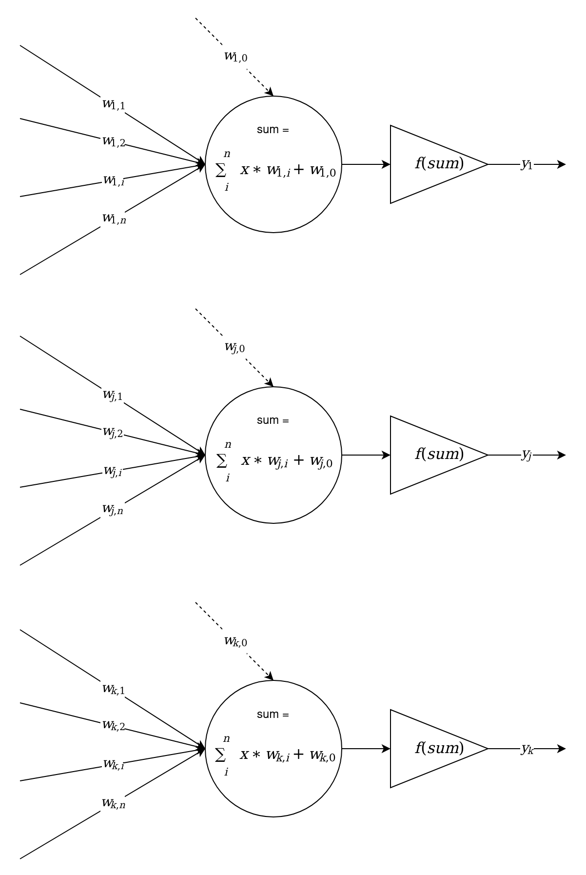
Currently, terms such as single-layer perceptron (SLP) (or just perceptron) and multilayer perceptron (MLP) are used. Usually, under the layers in the perceptron is a sequence of neurons, located at the same level and not connected. The following diagram shows this model:

Typically, we can distinguish between the following types of neural network layers:

• Input: This is just the source data or signals arriving as the input of the system (model). For example, these can be individual components of a specific vector from the training set, .
• Hidden: This is a layer of neurons located between the input and output layers. There can be more than one hidden layer.
• Output: This is the last layer of neurons that aggregates the model's work, and its outputs are used as the result of the model's work.

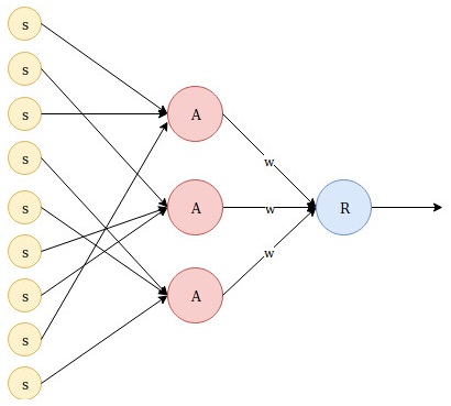
The term single-layer perceptron is often understood as a model that consists of an input layer and an artificial neuron aggregating this input data. This term is sometimes used in conjunction with the term Rosenblatt's perceptron, but this is not entirely correct since Rosenblatt used a randomized procedure to set up connections between input data and neurons to transfer data to a different dimension, which made it possible to the solve problems that arose when classifying linearly non-separable data. In Rosenblatt's work, a perceptron consists of S and A neuron types, and an R adder. S neurons are the input layers, A neurons are the hidden layers, and the R neuron generates the model's result. The terminology's ambiguity arose because the weights were used only for the R neuron, while constant weights were used between the S and A neuron types. However, note that connections between these types of neurons were established according to a particular randomized procedure:

The term MLP refers to a model that consists of an input layer, a certain number of hidden neurons layers, and an output layer. This can be seen in the following diagram:

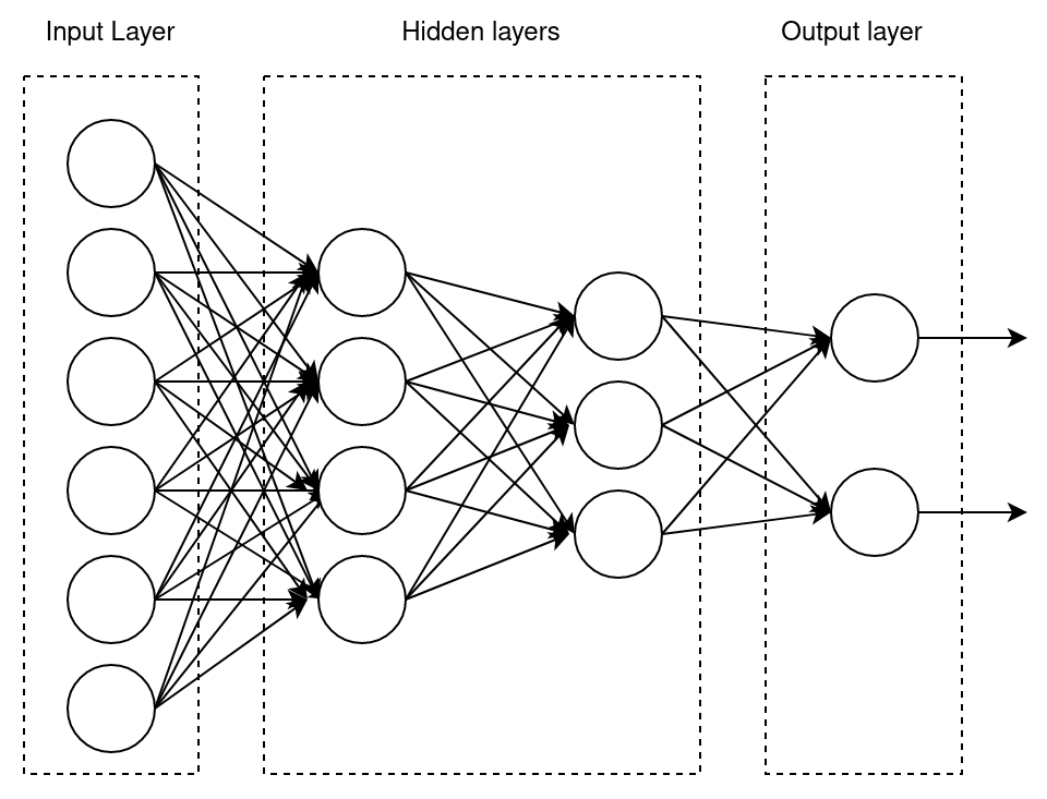
It should also be noted that the architecture of the perceptron (or neural network) includes the direction that signal propagation takes place in. In the preceding examples, all communications are directed strictly from the input neurons to the output ones – this is called a feedforward network. Other network architectures may also include feedback between neurons.

The second point that we need to pay attention to in the architecture of the perceptron is the number of connections between neurons. In the preceding diagram, we can see that each neuron in one layer connects to all the neurons in the next layer – this is called a fully connected layer. Such a connection is not a requirement, but we can see an example of a layer with different types of connections in the Rosenblatt perceptron scheme.

Now, let's learn how artificial neural networks can be trained.