Chapter 10: Data Modeling and Row-Level Security

In the previous chapter, we looked at the visual layer in Power BI, where a key point was to reduce the load on data sources by minimizing the complexity and number of queries. We learned that this area is usually the easiest and quickest place to apply performance-related fixes. However, experience working with a wide range of Power BI solutions has shown that issues with the underlying dataset are very common and typically have a greater negative performance impact. Importantly, this impact can be amplified because a dataset can be used by more than one report. Dataset reuse is a recommended practice to reduce data duplication and development effort.

Therefore, in this chapter, we will move one layer deeper, into modeling Power BI datasets with a focus on Import mode. Dataset design is arguably the most critical piece, being at the core of a Power BI solution and heavily influencing usability and performance. Power BI's feature richness and modeling flexibility provide alternatives when you're modeling data and some choices can make development easier at the expense of query performance and/or dataset size. Conversely, certain inefficient configurations can completely slow down a report, even with data volumes of far less than 1 GB.

We will discuss model design, dataset size reduction, building well-thought-out relationships, and avoiding pitfalls with row-level security (RLS). We will also touch on the tools and techniques we learned about in the previous chapters to look at the impact of design decisions.

In this chapter, we will cover the following topics:

• Building efficient data models
• Avoiding pitfalls with row-level security

Technical requirements

Some samples are provided in this chapter. We will specify which files to refer to. Please check out the Chapter10 folder in this book's GitHub repository to get these assets: https://github.com/PacktPublishing/Microsoft-Power-BI-Performance-Best-Practices.

Building efficient data models

We will begin with some theoretical concepts on how to model data for fast query performance. These techniques were designed with usability in mind but happen to be the perfect way to model data for the Analysis Services engine in Power BI. We will begin by introducing star schemas because they are native to the Analysis Services engine and it is optimized to work with them.

The Kimball theory and implementing star schemas

Data modeling can be thought of as how to group and connect the attributes in a set of data. There are competing schools of thought as to what style of data modeling is the best and they are not always mutually exclusive. Learning about competing data modeling techniques is beyond the scope of this book.

We will be looking at dimensional modeling, a very popular technique that was established by the Kimball Group over 30 years ago. It is considered by many to be an excellent way to present data to business users and happens to suit Power BI's Analysis Services engine very well. It can be a better alternative than trying to include every possible required field into a single wide table that's presented to the user. We recommend that you become more familiar with Kimball techniques as they cover the entire process of developing a BI solution, starting with effective requirements gathering. The group has published many books, all of which can be found on their website: https://www.kimballgroup.com.

Transactional databases are optimized for efficient storage and retrieval and aim to reduce data duplication via a technique called normalization. This can split related data into many different tables and requires joins on common key fields to retrieve the required attributes. For example, it is common for Enterprise Resource Planning suites to contain thousands of individual tables with unintuitive table and column names.

To deal with this problem, a central concept in the world of dimensional modeling is the star schema. Modeling data into star schemas involves designing data structures specifically for faster analysis and reporting but where we don't have to store the data efficiently. The simplest dimensional model consists of two types of tables:

• Fact: These tables contain quantitative attributes and record the business event's details, such as customer order line items or answers in a survey.
• Dimension: These tables contain qualitative attributes that help give the metrics context and are used to group and filter the data. Date and time periods such as quarter and month are the most obvious examples.

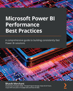
After defining the facts and dimensions in our model, we can see how the star schema gets its name. A simple star schema has a single fact table that's related to some dimensions tables that surround it, like the points of a star. This can be seen in the following diagram:

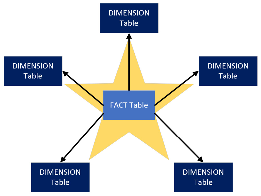
Figure 10.1 – A star schema

The preceding diagram shows a 5-pointed star simply for convenience to aid our conceptual learning. Note that there is technically no limit to how many dimensions you can include, though there are some usability considerations when there are too many. We'll look at a practical example of dimensional modeling in the next section.

Designing a basic star schema

Let's consider an example where we want to build a dimensional model to analyze employee leave bookings. We want to be able to determine the total hours they booked but also drill down to individual booking records to see how much time was booked and when the leave period starts. We need to identify the facts and dimensions and design the star schema. The Kimball group recommends a 4-step process to perform dimensional modeling. These steps are presented here, along with the results for our example scenario in parentheses:

1. Identify the business process (Leave booking).
2. Declare the grain (1 record per contiguous employee leave booking).
3. Identify the dimensions (Employee, Date).
4. Identify the facts (hours booked).

Now that we have completed the modeling process, let's look at a diagram of the star schema for this employee leave booking scenario. It contains the fact and dimensions we identified via the Kimball process. However, instead of two dimensions, you will see three related to the fact table. Date appears twice since we have two different dates to analyze – date booked versus start date. This is known as a role-playing dimension, another Kimball concept:

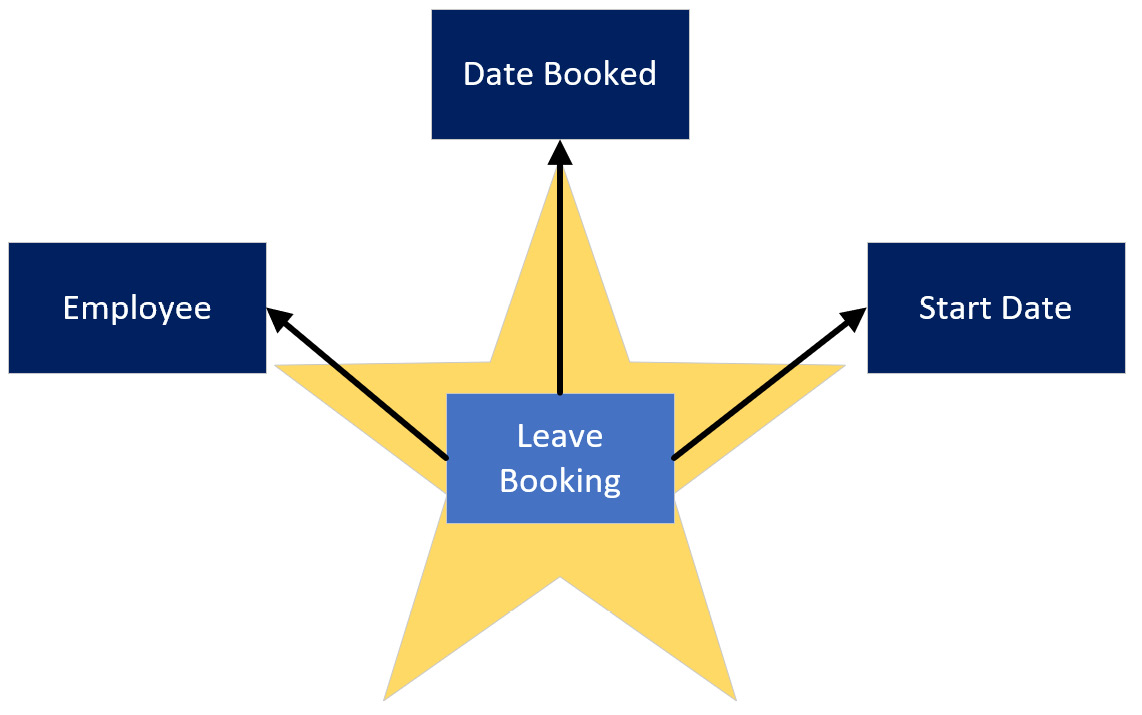
Figure 10.2 – Star schema for employee leave bookings

Steps one and two help determine our scope. The real work starts with step three, where we need to define the dimensions. With star schemas, we perform de-normalization and join some tables beforehand to bring the related attributes together into a single dimension table where possible. De-normalized tables can have redundant, repeated values.

Grouping values for a business entity makes for easier business analysis, and repetition isn't a problem for a column-storage engine such as Analysis Services, which is built to compress repeating data.

The concept of grouping can be seen in the following diagram, which shows normalized and de-normalized versions of the same employee data:

Figure 10.3 – De-normalizing three tables into a single employee dimension

In the preceding diagram, we can see that the RoleName attribute has been duplicated across the last two roles since we have two employees who are in the Analyst role.

A Date dimension simply contains a list of contiguous dates (complete years), along with date parts such as day of the week, month name, quarter, year, and so on. This is typically generated using a database script, M query, or DAX formulas. We won't illustrate these details as they are not relevant to our example.

The final step is to model the fact table. Since we determined that we want one row per employee leave booking, we could include the following attributes in the fact table:

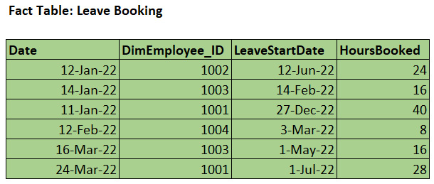
Figure 10.4 – Leave Booking fact table

Note

We have provided a trivial example of a business problem for dimensional modeling in this book to aid learning. Note that dimensional modeling is a unique discipline and it can be significantly more complex in some scenarios. There are different types of dimension and fact tables and even supplementary tables that can solve granularity issues. We will briefly introduce a few of these more advanced modeling topics, though we encourage you to perform deeper research to learning about these areas if needed.

Next, we will look at one advanced data modeling topic that has specific relevance to Power BI.

Dealing with many-to-many relationships

An important Kimball concept that has specific relevance to Power BI is that of many-to-many relationships, which we will abbreviate as M2M. This type of relationship is used to model a scenario where there can be duplicate values in the key columns on both sides of the relationship. For example, you may have a table of target or budget values that are set at the monthly level per department, whereas other transactions are analyzed daily. The latter requirement determines that the granularity of the date dimension should be daily. The following screenshot shows some sample source data for such a scenario. It highlights the YearMonth field, which we need to use to join the tables at the correct granularity, and that there are duplicate values in both tables:

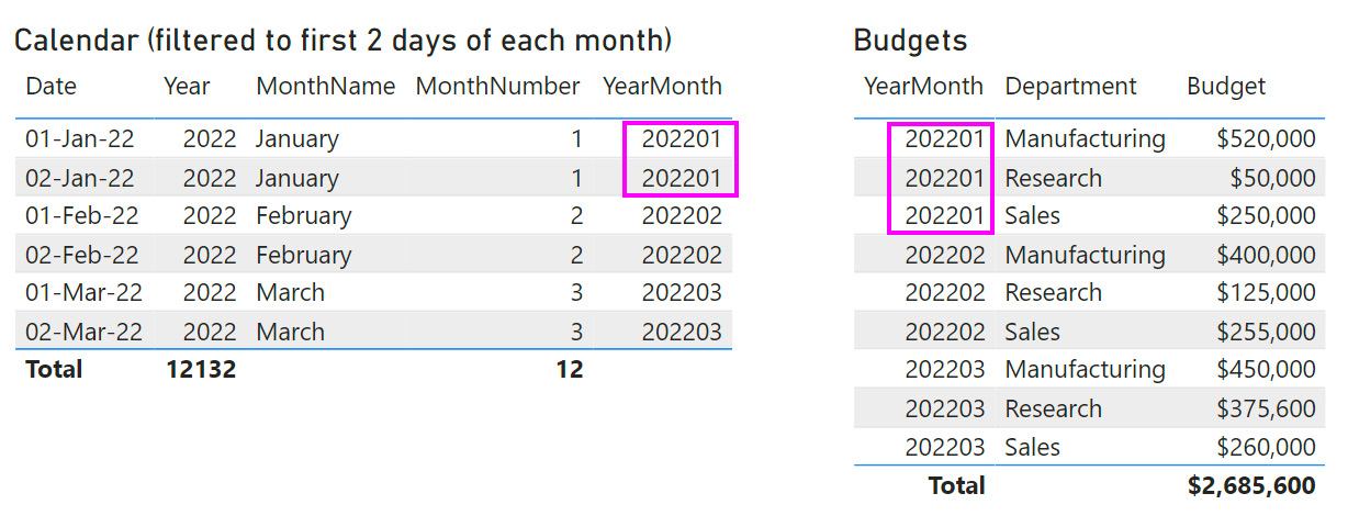
Figure 10.5 – Calendar and Budgets data showing duplicates in the key column

This preceding diagram demonstrates a completely legitimate scenario that has different variations. When you try to build a relationship between columns with duplicates in Power BI, you will find that you can only create a Many to many type, as shown in the following screenshot:

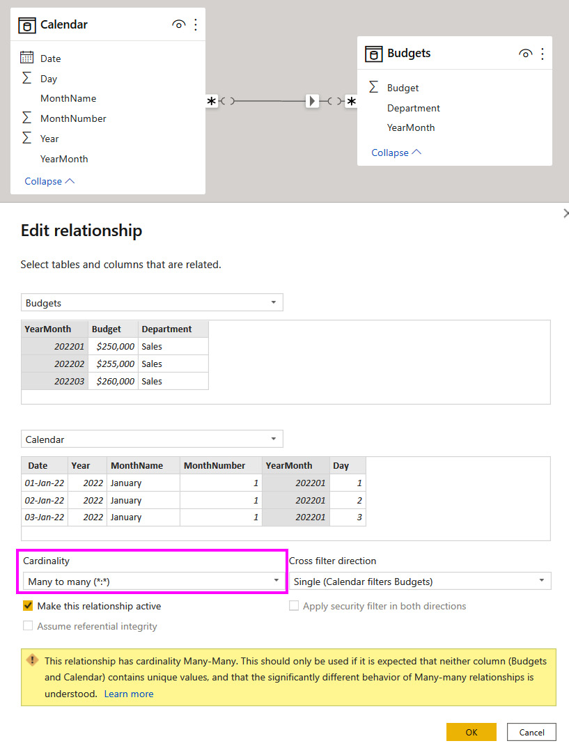
Figure 10.6 – Many-to-many relationship configuration

Once the M2M relationship has been configured, Power BI will resolve the duplication and display the correct results in visuals. For example, if you show the total Budget values using Year from the Calendar table, the sums will be correct, as shown in the following screenshot:

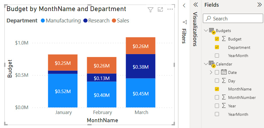
Figure 10.7 – Correct results with the M2M relationship type

Now that we have described when and how to use M2M relationships, we advise using them with care and generally with smaller datasets.

Important Note

The M2M relationship type should be avoided when you're dealing with large datasets, especially if there are many rows on both sides of the relationship. The performance of this relationship type is slower than the more common one-to-many relationships and can degrade more as data volumes and DAX complexity increase. Instead, we recommend employing bridge tables to resolve the relationship into multiple one-to-many relationships. You will also need to adjust the measures slightly. This approach will be described shortly.

You can avoid the performance penalty of using an M2M relationship by adding a new table to the dataset called a bridge table. The following screenshot shows how we can introduce a bridge table between the Calendar and Budgets tables with all the relationships being one-to-many. The bridge table simply contains pairs of keys that can connect unique rows from each table. So, we need to introduce a BudgetKey field to the Budgets table to uniquely identify each row:

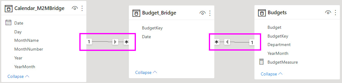
Figure 10.8 – A bridge table added with only one-to-many relationships

A small change is required to ensure the bridge tables work correctly with calculations. We need to wrap any measure around a CALCULATE() statement that explicitly filters over the bridge table. In our case, we can hide the Budget column and replace it with a calculation, as shown here:

BudgetMeasure = CALCULATE(SUM(Budgets[Budget]), Budget_Bridge)

You can see both techniques in action in the sample Many to many.pbix file that's included with this chapter.

In our trivial example with a small number of rows, creating a bridge table would seem like an unnecessary effort, and it even introduces more data into the model. The performance benefit is likely to be negligible and using the M2M relationship type would be better for easier maintenance. However, as data volumes grow, we recommend implementing bridge tables and doing a performance comparison over typical reporting scenarios.

Next, we will learn how to reduce dataset size, which helps with the performance of refresh and report viewing.

Reducing dataset size

In Chapter 2, Exploring Power BI Architecture and Configuration, we learned that the import mode tables in a Power BI dataset are stored in a proprietary compressed format by Analysis Services. We should aim to keep these tables as small as possible to reduce both data refresh and query durations by having fewer data to process. There is also the initial dataset load to consider. Power BI does not keep every dataset in memory all the time for practical reasons. When a dataset has not been used recently, it must be loaded from disk into memory the next time someone needs it. This initial dataset load duration increases as the dataset's size increases.

The benefits of smaller datasets are beyond just speed. In general, fewer data to process means less CPU and memory usage, which benefits the overall environment by leaving more resources available for other processes.

The following techniques can be used to reduce dataset size:

• Remove unused tables and columns: If any table or column elements are not needed anywhere in the dataset or downstream reports, it is a good idea to remove them from the dataset. Sometimes, tables or attributes are used for calculations and not exposed to users directly, so these can't be removed easily.
• Avoid high precision and high cardinality columns: Sometimes, source data may be stored in a format that supports a much higher precision than we would ever need for our analysis. For example, a date column to the second is not required if we only ever analyze per day at the highest granularity. Similarly, the weight of a person to 2 decimal places might not be needed if we always plan to display them as a whole number. Therefore, we recommend reducing the precision in Power Query, in a pushed-down transformation, or permanently in the original data source if that's feasible and safe. Let's build on the decimal versus whole number example. Power BI stores both types as a 64-bit value that occupies 8 bytes. Initially, this won't seem like it makes a difference in terms of storage. This is true, though the dataset size reductions will be realized because we are reducing the number of unique values with lower precision (for example, all the values between 99.0 and 99.49 collapse to 99 when we reduce the precision). Fewer unique values will reduce the size of the internal dictionary.

The same concept extends to high cardinality columns. Cardinality means the number of unique elements in a group. A high cardinality column will have few repeated values and will not compress well. Sometimes, you will already know that every value in a column is unique. This is typical of row identifiers or primary keys such as an employee ID, which are unique by design. Be aware that you may not be able to remove unique columns because they are essential for relationships or report visuals.

• Disable auto date/time: If you have many date columns in your dataset, a lot of space may be taken up by the hidden date tables that Power BI automatically creates. Be sure to disable this setting in Power BI Desktop, as described in Chapter 2, Exploring Power BI Architecture and Configuration.
• Split datetime into date and time: If you need to perform analysis with both date and time, consider splitting the original datetime attribute into two values – that is, date only and time only. This reduces the total number of unique date elements. If we had 10 years of data to analyze and designed a date table to the second granularity, we would have about 315 million unique datetime entries (10 years x 365 days x 24 hours x 60 minutes x 60 seconds). However, if we split this, we would only get 90,050 unique items – that is, a table of unique dates with 10 x 365 entries, and a table of unique times with 24 x 60 x 60 entries. This represents a raw row count reduction of over 99%.
• Replace GUIDs with surrogate keys for relationships: A GUID is a Globally Unique Identifier consisting of 32 hexadecimal characters separated by hyphens. An example of this is 123e4567-e89b-12d3-a456-426614174000. They are stored as text in Analysis Services. Relationships across text columns are not as efficient as those across numerical columns. You can use Power Query to generate a surrogate key that will be substituted for the GUID in both the dimension and fact tables. This could be resource and time-intensive for large datasets, trading off refresh performance for query performance. An alternative is to work with database or data warehouse professionals to have surrogate keys provided at the source if possible. This technique does cause problems if the GUID is needed. For example, someone may want to copy the ID value to look up something in an external system. You can avoid preloading the GUID in the dataset by using a composite model and a report design that provides a drilling experience to expose just one or a small set of GUIDs on-demand via DirectQuery. We will cover composite models in more detail in Chapter 12, High-Scale Patterns.
• Consider composite models or subsets for very large models: When you have models that approach many tens or even hundreds of tables, you should consider creating subsets of smaller datasets for better performance. Try to include only facts that are highly correlated from a business perspective and that need to be analyzed by the same type of user in a single report visual, page, or analytical session. Avoid loading facts that have very few dimensions in common into the same dataset. For example, leave bookings and leave balances would likely belong to the same dataset, whereas leave bookings and website inquiries would likely not. You can also solve such problems using aggregations and composite models, which we will also discuss in Chapter 12, High-Scale Patterns. This tip also applies to slow DirectQuery models, where moving to composite models with aggregations can provide significant performance benefits.
• Use the most efficient data type, and integers instead of text: Power BI will try to choose the right data types for columns for you. If data comes from a strongly-typed source such as a database, it will match the source data type as closely as possible. However, with some sources, the default that's chosen may not be the most efficient, so it's worth checking. This is especially true for flat files, where whole numbers might be loaded as text. In such cases, you should manually set the data type for these columns to integers because integers use value encoding. This method compresses more than dictionary encoding and run-length encoding, which are used for text. Integer relationships are also faster.
• Pre-sort integer keys: Power BI scans values in columns as they are read, row by row. It samples rows to decide what type of compression to apply. This compression is performed on groups of rows called segments. Currently, SQL Server and Azure Analysis Services work with 8 million row segments, while Power BI Desktop and the Power BI Service work with 1 million row segments. For larger tables, it is worth loading the data into Power BI with the keys already sorted. This will reduce the range of values per segment, which is beneficial for run-length encoding.
• Use bi-directional relationships carefully: This type of relationship allows slicers and filter context to propagate in either direction across a relationship. If a model has many bi-directional relationships, applying a filter condition to a single part of the dataset could have a large downstream impact as all the relationships must be followed to apply the filter. Traversing all the relationships is extra work that could slow down queries. We recommend only turning on bi-directional relationships when the business scenario requires it.
• Offload DAX calculated columns: Calculated columns do not compress as well as physical columns. If you have calculated columns, especially with high cardinality, consider pushing the calculation down to a lower layer. You can perform this calculation in Power Query. Aim to leverage pushdown here too, using guidance from Chapter 8, Loading, Transforming, and Refreshing Data.
• Set the default summarization: Numeric columns in a Power BI dataset usually default to the Sum aggregation, and occasionally to the Count aggregation. This property can be set in the Data tab of Power BI Desktop. You may have integers that do not make sense to aggregate, such as a unique identifier such as an order number. If the default summarization is set to Sum, Power BI will try to sum this attribute in visuals. This may confuse users, but for performance, we are concerned that we are doing meaningless sums. Therefore, we advise reviewing the summarization settings, as shown in the following screenshot:

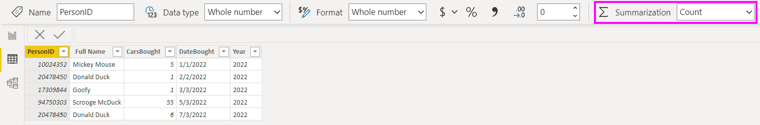
Figure 10.9 – Summarization on an identifier column set to Count instead of Sum

Next, we will look at optimizing RLS for datasets.

Avoiding pitfalls with row-level security (RLS)

RLS is a core feature of Power BI. It is the mechanism that's used to prevent users from seeing certain data in the dataset. It works by limiting the rows that a user can access in tables by applying DAX filter expressions.

There are two approaches to configuring RLS in Power BI. The simplest RLS configuration involves creating a role in the dataset, then adding members, which can be individual users or security groups. Then, DAX table filter expressions are added to the role to limit which rows members can see. A more advanced approach, sometimes referred to as dynamic RLS, is where you create security tables in the dataset that contain user and permission information. The latter is often used when permissions can change often, and it allows the security tables to be maintained automatically, without the Power BI dataset needing to be changed. We assume you are familiar with both approaches.

Performance issues can arise when applying filters becomes relatively expensive compared to the same query with no RLS involved. This can happen when the filter expression is not efficient and ends up using the single-threaded formula engine, which we learned about in Chapter 6, Third-Party Utilities. The filter may also be spawning a lot of storage engine queries.

Let's begin by providing some general guidance for RLS configuration:

• Perform RLS filtering on dimension tables rather than fact tables: Dimensions generally contain far fewer rows than facts, so applying the filter the dimension allows the engine to take advantage of the much lower row count and relationships to perform the filtering.
• Avoid performing calculations in the DAX filter expression, especially string manipulation: Operations such as conditional statements and string manipulations are formula engine bound and can become very inefficient for large datasets. Try to keep the DAX filter expressions simple and try to adjust the data model to pre-calculate any intermediate values that are needed for the filter expression. One example is parent-child hierarchies, where a table contains relationship information within it because each row has a parent row identifier that points to its parent in the same table. Consider the following example of a parent-child dimension for an organizational structure. It has been flattened with helper columns such as Path beforehand so that DAX calculations and security can be applied to the levels. This approach is typical in Power BI for handling a parent-child situation:

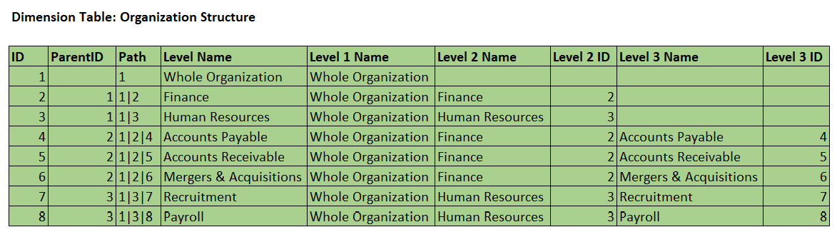
Figure 10.10 – A typical parent-child dimension configured for Power BI

Suppose we wanted to create a role to give people access to all of Finance. You might be tempted to configure a simple RLS expression, like so:

PATHCONTAINS('Organization Structure'[Path], 2)

This will work, but it does involve string manipulation because the function is searching for a character in the Path column. For better performance, the following longer expression is preferred because it only compares integers:

'Organization Structure'[Path] = 2

• Optimize relationships: Security filters are applied from dimensions to facts by following relationships, just like any regular filter that's used in a report or query. Therefore, you should follow the relationship best practices that were mentioned in the previous section and Chapter 3, DirectQuery Optimization.
• Test RLS in realistic scenarios: Power BI Desktop allows you to simulate roles to test RLS. You should use tools such as Desktop Performance Analyzer and DAX Studio to capture durations and engine activity with and without RLS applied. Look for differences in formula engine durations and storage engine query counts to see what the impact of the RLS filter is. It also is recommended to test a published version in the Power BI service with a realistic production data volume. This can help identify issues that may not be caught in development with smaller data volumes. Remember to establish baselines and measure the impact of individual changes, as recommended in Chapter 7, Governing with a Performance Framework. For a good instructional video that covers testing various forms of RLS with the tools we covered in Chapter 3, DirectQuery Optimization, we recommend checking out the following video, which was published by Guy in a Cube: https://www.youtube.com/watch?v=nRm-yQrh-ZA.

Next, let's look at some guidance that applies to dynamic RLS:

• Avoid unconnected security tables and LOOKUPVALUE(): This technique simulates relationships by using a function to search for value matches in columns across two tables. This operation involves scanning through data and is much slower than if the engine were to use a physical relationship, which we recommend instead. You may need to adjust your security table and data model to make physical relationships possible, which is worth the effort.
• Keep security tables as small as possible: With dynamic RLS, the filter condition is initially applied to the security tables, which then filter subsequent tables via relationships. We should model the security tables to minimize the number of rows they contain. This minimizes the number of potential matches and reduces engine filtering work. Bear in mind that a single security table is not a Power BI requirement, so you are not forced to combine many permissions and grains into a large security table. Having a few small security tables that are more normalized can provide better performance.
• Avoid using bi-directional security filters: Security filter operations are not cached when they're bi-directional, which results in lower performance. If you must use them, try to limit the security tables to less than 128,000 rows.
• Collapse multiple security contexts into a single security table: If you have many different RLS filters from dimensions being applied to a single fact table, you can build a single security table using the same principles as the Kimball junk dimension. This can be a complete set of every possible combination of permissions (also known as a cross-product) or just the actual unique permission sets that are required by users. A cross-product is very easy to generate but can result in combinations that do not make sense and can never exist.

To see this technique in practice, let's consider the following setup, where one fact table is being filtered by multiple dimensions with security applied. The arrows represent relationships and the direction of filter propagation:

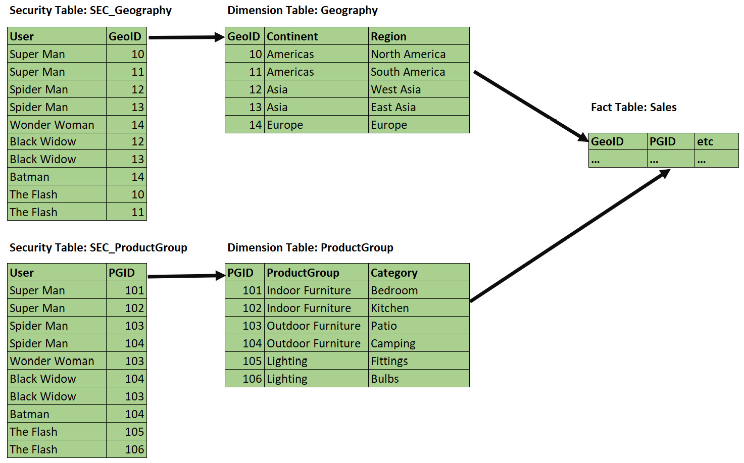
Figure 10.11 – Securing a single fact via multiple dimensions

We could reduce the amount of work that's needed to resolve security filters by combining the permissions into a single security table, as shown in the following screenshot:

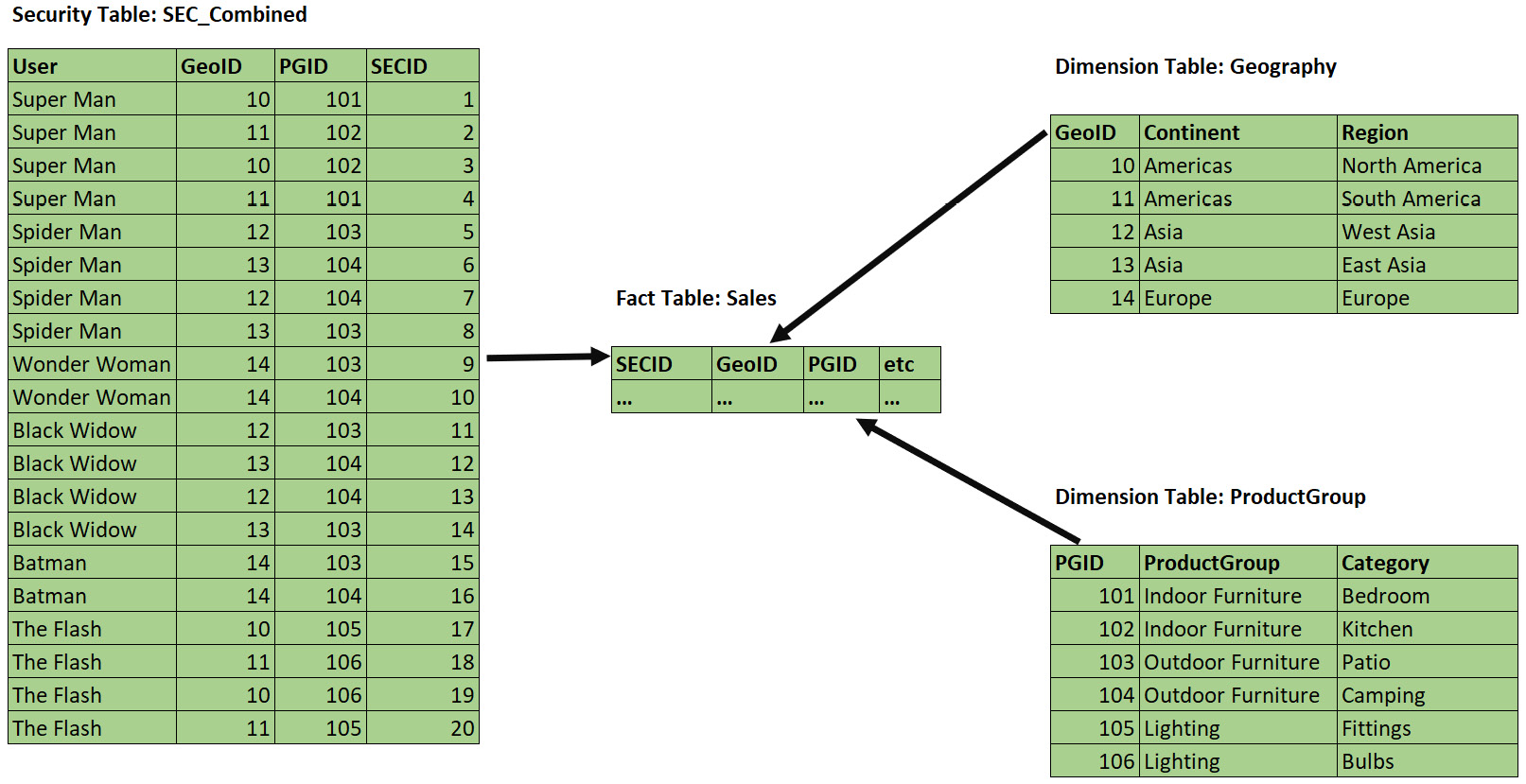
Figure 10.12 – More efficient configuration to secure a single fact

Note that our SEC_Combined table does not use a cross-product – it only contains valid combinations that exist in the source data, which will result in a smaller table. This is preferred when you have many dimensions and possible values. In our trivial example, the table contains 20 rows instead of the 30 combinations that would come from a cross-product (5 Geography rows x 6 ProductGroup rows).

You can see the effect of this change by running some report pages or queries with and without RLS applied, as described earlier. Check out RLS.pbix and RLS Combined.pbix in the sample files to see these in action. They contain the configurations from Figure 10.10 and Figure 10.11, respectively, with a single fixed role to simulate the Super Man user.

We ran some tests in DAX Studio using a role built for Super Man and got the results shown in the following table. Even though we only had 25,000 rows, and the durations were trivial, you can already see a 300% difference in the total duration when RLS is applied using the combined approach. With many users, dimensions, and fact rows, this difference will be significant and noticeable in reports:

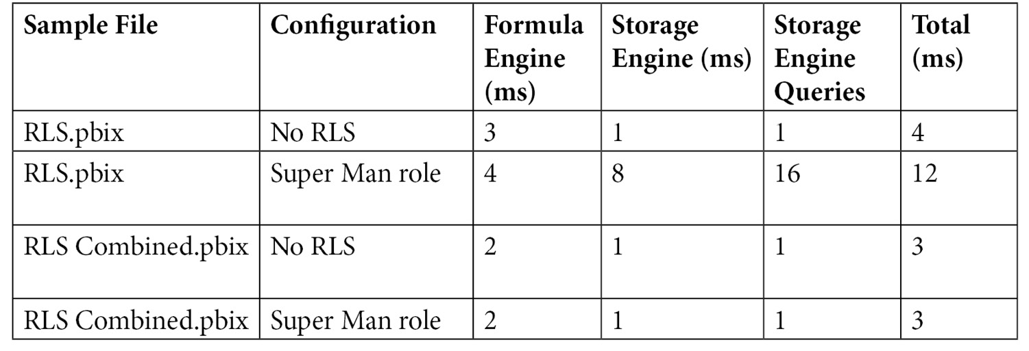
Figure 10.13 – Performance comparison of different RLS configurations

• Combine multiple users with the same security context: In Figure 10.11, our security table contains multiple rows per user and some duplicate permission sets. For example, observe that both Spider Man and Black Widow have access to all of Asia and Outdoor Furniture. If you have many hundreds or thousands of users, security tables like this can get quite large. If users have the same permission sets, we can reduce the size significantly by performing modeling, as shown for the Geography dimension in the following screenshot. Observe how we have two much smaller security tables. Also, note the appropriate use of M2M and bi-directional filters by exception here – performance can improve massively with this setup when used correctly:

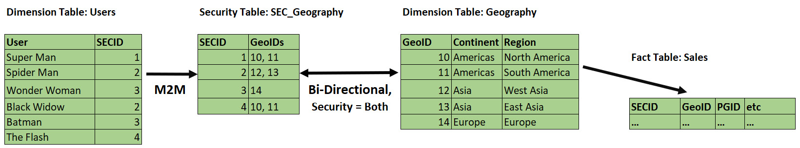
Figure 10.14 – Combining multiple users and permissions

Building specialized security tables like the one shown in the preceding screenshot can be achieved in different ways. You could build the tables externally as part of regular data warehouse loading activities, or you could leverage Power Query.

Now, let's summarize what we've learned in this chapter.

Summary

In this chapter, we learned how to speed up Power BI datasets in Import mode. We began with some theory on Kimball dimensional modeling, where we learned about star schemas, which are built from facts and dimensions. Data modeling is about grouping and relating attributes, and star schemas are one way to model data. They provide non-technical users with an intuitive way to analyze data by combining qualitative attributes into dimension tables. These dimensions are related to fact tables, which contain qualitative attributes. Power BI's Analysis Services engine works extremely well with star schemas, which are preferred. Hence, we briefly looked at the four-step dimensional modeling process and provided a practical example, including one with many-to-many relationships.

Then, we focused on reducing the size of datasets. This is important because less data means less processing, which results in better performance and more free resources for other parallel operations. We learned how to exclude any tables and columns that aren't needed for the report or calculations. We also explored techniques to help Analysis Services compress data better, such as choosing appropriate data types, reducing cardinality for columns, and preferring numbers over text strings.

Lastly, we learned how to optimize RLS. We learned that RLS works just like regular filters and that previous guidance about fast relationships also applies to RLS. The main thing to remember with RLS is to keep DAX security filter expressions as simple as possible, especially to avoid string manipulation. With dynamic RLS, we use security tables and we learned to keep the security table as small as possible. We also taught you how to use Desktop Performance Analyzer and DAX Studio to capture queries and look at performance before and after RLS is applied.

In the next chapter, we will look at DAX formulas, where we will identify common performance traps and suggest workarounds.