Chapter 12: High-Scale Patterns

In the previous chapter, we learned how to optimize DAX expressions. Having reached this point, we have rounded up all the advice on optimizing different layers of a Power BI solution, from the dataset layer to report design. In this chapter, we will take a step back and revisit architectural concepts and related features that help deal with very high data volumes.

The amount of data that organizations collect and need to analyze is increasing all the time. With the advent of the Internet of Things (IoT) and predictive analytics, certain industries, such as energy and resources, are collecting more data than ever. It is common for a modern mine or gas plant to have tens of thousands of sensors, each generating many data points at granularities much higher than a second.

Even with Power BI's data compression technology, it isn't always possible to load and store massive amounts of data in an Import mode model in a reasonable amount of time. This problem is worse when you must support hundreds or thousands of users in parallel. This chapter will cover the options you have for dealing with such issues by leveraging composite data models and aggregations, Power BI Premium, and Azure technologies. The concepts in this chapter are complementary and can be combined in the same solution as appropriate.

In this chapter, we will cover the following topics:

• Scaling with Power BI Premium and Azure Analysis Services
• Scaling with composite models and aggregations
• Scaling with Azure Synapse and Data Lake

Technical requirements

There is a combined sample file available for this chapter. All the sample references can be found in the Composite and Aggs.pbix file, in the Chapter12 folder in this book's GitHub repository: https://github.com/PacktPublishing/Microsoft-Power-BI-Performance-Best-Practices. Since this example uses DirectQuery to access a SQL server database, we have included the AdventureWorksLT2016.bak SQL backup. Please restore that database to a SQL server and update the connection in Power BI Desktop to run the sample successfully.

Scaling with Power BI Premium and Azure Analysis Services

Power BI users with Pro licenses can create workspaces in the Shared or Premium capacity. Shared capacity is available by default to any organization using Power BI. Shared capacity is managed entirely by Microsoft, which load balance multiple tenants over thousands of physical machines around the world. To provide a consistent and fair experience for everyone, there are certain limits in Shared capacity. One that affects data volumes is the 1 GB size limit of a compressed dataset. Power BI Desktop will allow you to create datasets that are only limited by the amount of memory on the computer, but you will not be allowed to upload a dataset that's larger than 1 GB to Shared capacity. Similarly, if a dataset hosted in Shared capacity grows to over 1 GB, it will result in refresh errors. Note that this limit refers to the compressed data size, so the actual source data can be many times larger.

Leveraging Power BI Premium for data scale

One way to resolve the Shared dataset size limit issue is to leverage dedicated capacity via Power BI Premium. Premium capacity must be purchased separately, and the computing resources are dedicated to the organization. Customers can purchase Premium capacity of different sizes, ranging from P1 (8 cores and 25 GB of RAM) to P5 (128 cores and 400 GB of RAM). Also, note that Microsoft offers Power BI Embedded capacities. While these are licensed, purchased, and billed differently from the Premium capacities, the technology is the same and any advice given here applies to both Premium and Embedded.

Premium capacity offers a range of unique features, higher limits, and some enhancements that help with performance and scale. We will cover Premium optimization in detail in Chapter 13, Optimizing Premium and Embedded Capacities. For now, the important point is that the dataset limit in Premium is raised to 10 GB. However, this is just the limit of the initial dataset that is uploaded to the Premium capacity.

Tip

If your dataset will grow beyond 1 GB in size, you should consider using Power BI Premium. Power BI Premium will allow you to upload a dataset up to a maximum size of 10 GB that can grow to 12 GB after being refreshed. However, if you choose the large dataset format, the dataset will have no size limit. The available capacity memory is the only limiting factor. You can even provision multiple Premium capacities of different sizes and spread your load accordingly. Always plan to have free memory on the capacity to handle temporary storage for queries, which can include uncompressed data. Lastly, the large dataset format can also speed up write operations that are performed via the XMLA endpoint.

The following screenshot shows the Large dataset storage format setting on a published dataset. It is part of the Dataset settings page and can be accessed from a Power BI workspace. You can enable this to remove the dataset's size limit:

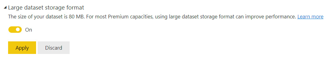
Figure 12.1 – Large dataset storage format option in Dataset settings

Be aware that you can set the large dataset storage format to be the default on a Premium capacity. Administrators can set a limit on the maximum dataset size to prevent users from consuming significant amounts of a capacity.

With the large dataset format, Premium is an excellent choice to handle data scale. It can also support more users simply by having more computing resources available on the platform that can handle more concurrent queries and, therefore, users. The ability to provision multiple capacities also provides user-scale benefits since you can avoid having very popular datasets in the same capacity.

However, you may still have a scenario where you have extreme data volumes with many concurrent users that are pushing a Premium capacity to its limits. Next, we will learn how to deal with this problem with Azure Analysis Services.

Leveraging Azure Analysis Services for data and user scale

Azure Analysis Services (AAS) is a Platform-as-a-Service (PaaS) offering. It is part of the broader suite of data services offered by Microsoft in the Azure cloud. A range of SKUs are available, with processing power stated in Query Processing Units (QPU).

AAS can be considered as the cloud alternative to SQL Server Analysis Services. For organizations that already use SQL Server Analysis Services and want to migrate to the cloud, AAS is the best option and offers the most direct migration path. AAS is billed on a pay-as-you-go basis, can be paused and scaled on demand, and offers comprehensive support for Power BI Pro developer tools such as Microsoft Visual Studio with version control and the ability to perform Continuous Integration/Continuous Development (CI/CD). Like SQL Server Analysis Services, AAS is the data engine only, so it only supports hosting datasets and the mashup engine. You would still need to use a client tool such as Power BI Desktop or a portal such as PowerBI.com to host reports that read from AAS. AAS can be considered a subset of Premium, though this is not completely true today. This is because there are differences, such as dynamic memory management, which is only offered in Premium, and Query Scale Out (QSO), which is only available in AAS (Standard tier). QSO is a great way of handling high user concurrency with minimal maintenance, so it is a pity to not have it available in Premium today. However, it is encouraging to note that Microsoft has stated their intention to have Premium become a true superset of AAS.

Using Query Scale Out to achieve higher user concurrency

Power BI Premium and AAS have the same dataset size limits, so you can host the same data volumes on either. However, QSO is a unique capability of AAS that allows it to handle many more concurrent users by spreading the query read load across multiple redundant copies of the data. You simply configure the service to create additional read replicas (up to a maximum of 7 additional replicas). When client connections are made, they are load-balanced across query replicas. Note that not every region and SKU supports 7 replicas, so please consult the documentation for information on availability by region at https://docs.microsoft.com/azure/analysis-services/analysis-services-overview. Also, please note that replicas do incur costs, so you should consider this aspect when you review your performance gains.

Another useful performance-related feature of AAS is its ability to separate the query and processing servers when we use QSO. This maximizes the performance of both processing and query operations. The separation means that at refresh time, one of the replicas will be dedicated to the refresh and no new client connections will be assigned to it. New connections will be assigned to query replicas only so that they can handle reads while the processing replica can handle writes.

Configuring replicas can be done via the Azure portal or scripted via PowerShell. The following screenshot shows an example where we are allowed to create one additional replica:

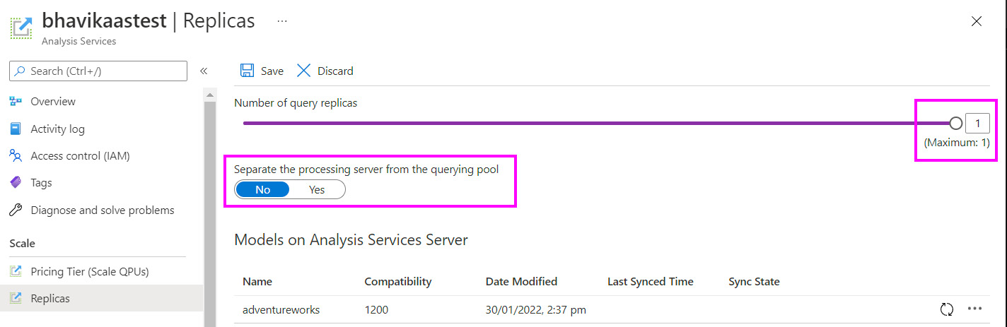
Figure 12.2 – AAS server with 1 replica highlighting the query pool separation setting

Note that creating replicas does not allow you to host larger datasets than if you were not using QSO. It simply creates additional identical copies with the same server SKU.

Lastly, let's talk about how to determine the right time to scale out. You can observe AAS metrics in the Azure portal to look at QPU over time. If you find that you regularly reach the maximum QPU of your service and that those time frames are correlated with performance issues, it is time to consider QSO. The following screenshot shows the QPU metric for an S0-sized AAS server that has a QPU limit of 40. We can see that we are not hitting that limit right now:

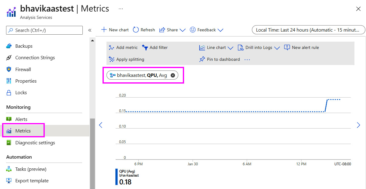
Figure 12.3 – Metrics in the Azure portal showing QPU over time

Next, we'll learn how partitions can improve refresh performance.

Using partitions with AAS and Premium

AAS has supported partitioned tables for many years. Partitions simply divide a table into smaller parts that can be managed independently. Typically, partitioning is done by date and is applied to fact tables. For example, you could have 5 years of data split into 60 monthly partitions. In this case, you could process individual partitions separately and even perform entirely different operations on them, such as clearing data from one while loading data into another.

From a performance perspective, partitions can speed up data refresh operations in two ways:

• Firstly, you can only process new and updated data by leaving historical partitions untouched and avoiding a full refresh.
• Secondly, you can get better refresh performance since partitions can be processed in parallel.

Maximum parallelism assumes that there is sufficient CPU power and memory available in AAS and that the data source can support the load. AAS automatically utilizes parallel processing for two or more partitions and there are no associated configuration settings for it.

Tip

Power BI Premium (with a large dataset storage format) and AAS use a segment size of 8 million rows. Segments are the internal structures that are used to split columns into manageable chunks, and compression is applied at the segment level. Therefore, we recommend employing a strategy where partitions have at least 8 million rows when fully populated. This will help AAS get the best compression and avoid doing extra maintenance work on many small partitions. Over-partitioning can slow down a dataset refresh and result in slightly larger datasets.

Tables defined in a Power BI dataset have a single partition by default. You cannot directly control partitioning in Power BI Desktop. However, note that when you configure incremental refreshes, partitions are automatically created and managed based on your time granularity and data freshness settings.

So, when we're using AAS or Power BI Premium, we need to define partitions manually using other tools. Partitions can be defined at design time in Visual Studio using the Partition Manager screen. Post-deployment, they can be managed using SQL Server Management Studio by running Tabular Model Scripting Language (TMSL). You can also manage them programmatically via the Tabular Object Model (TOM).

You can control parallelism at refresh time by using the TMSL parameter called MaxParallelism, which limits the total number of parallel operations, regardless of the data source. Some sample code for this was provided in the first section of Chapter 8, Loading, Transforming, and Refreshing Data.

Earlier in this section, we described a simple approach that used monthly partitions. A more advanced approach could be to have yearly or monthly historical partitions with daily active partitions. This provides you with a lot more flexibility to update recent facts and minimize re-processing if refresh failures occur since you can re-process at the single-day granularity. However, this advanced strategy requires extra maintenance since partitions would need to be merged. For example, at the end of each month, you may merge all the daily partitions into a monthly one. Performing this type of maintenance manually can become tedious. Therefore, it is recommended that you automate this process with the help of some tracking tables to manage date ranges and partitions. A detailed automated partition management sample has been published by Microsoft that we recommend: https://github.com/microsoft/Analysis-Services/blob/master/AsPartitionProcessing/Automated%20Partition%20Management%20for%20Analysis%20Services%20Tabular%20Models.pdf.

The final performance-related point is about synchronization mode for query replicas. When datasets are updated, the replicas that are used for QSO also need to be updated to give all the users the latest data. By default, these replicas are rehydrated in full (not incrementally) and in stages. Assuming there are at least three replicas, they are detached and attached two at a time, which can disconnect some clients. This behavior is determined by a server property called ReplicaSyncMode. It is an advanced property that you can set using SQL Server Management Studio, as shown in the following screenshot. This setting can be changed to make synchronization occur in parallel. Parallel synchronization updates in-memory caches incrementally and can significantly reduce synchronization time. It also provides the benefit of not dropping any connections because replicas are always kept online:

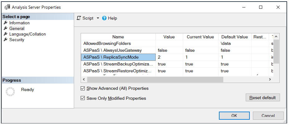
Figure 12.4 – Analysis Server Properties showing that ReplicaSyncMode has been updated

The following settings for ReplicaSyncMode are allowed:

• 1: Full rehydration performed in stages. This is the default.
• 2: Parallel synchronization.

  Note

  When using parallel synchronization, additional memory may be consumed by query replicas because they stay online and are still available for queries. The synchronization operation behaves like a regular data refresh, which could require double the dataset memory for a full refresh, as discussed in Chapter 2, Exploring Power BI Architecture and Configuration.

In the next section, we'll learn how to take advantage of composite models in Power BI to address big data and slow DirectQuery problems.

Scaling with composite models and aggregations

So far, we have discussed how Import mode offers the best possible speed for Power BI datasets. However, sometimes, high data volumes and their associated refresh limitations may lead you to select DirectQuery mode instead. At this point, you may want to review the Choosing between Import and DirectQuery mode section on choosing a storage mode in Chapter 2, Exploring Power BI Architecture and Configuration, to remind yourself about the differences and rationale for choosing one over the other.

We also discussed how the Analysis Services engine is designed to aggregate data efficiently because BI solutions typically aggregate data most of the time. When we use DirectQuery, we want to push these aggregations down to the source where possible to avoid Power BI having to bring all the data over to compute them. With very large tables containing tens of millions to billions of rows, these aggregations can be costly and time-consuming, even when the source has been optimized. This is where the composite models and aggregations features become relevant.

Leveraging composite models

So far, we have talked about the Import and DirectQuery modes separately. This may have implied that you must choose only one mode, but this is not the case. A composite model (also known as Mixed mode) is a feature of Analysis Services that lets you combine DirectQuery and Import data sources in the same dataset. This opens up interesting possibilities. You could enhance a DirectQuery source with infrequently changing Import data that is held elsewhere. You can even combine different DirectQuery sources. Regardless of the requirement, you are advised to follow all the recommended guidelines we have provided for Import and DirectQuery to date. There are some additional performance concepts and considerations for composite models that we will introduce in the remainder of this chapter.

Analysis Services maintains storage mode at the table level. This allows us to mix storage modes within a dataset. The bottom-right corner of Power BI Desktop gives us an indication of the type of model. An Import mode model will not show any status, but DirectQuery and Composite will show some text, as shown in the following screenshot:

Figure 12.5 – Power BI Desktop indicating the DirectQuery or Mixed (composite) storage mode

There are different ways to achieve Mixed mode in Power BI Desktop. You could add a new table in Import mode to an existing DirectQuery model, or vice versa. Another way is to directly change the storage mode in the Model view of Power BI Desktop, as shown here:

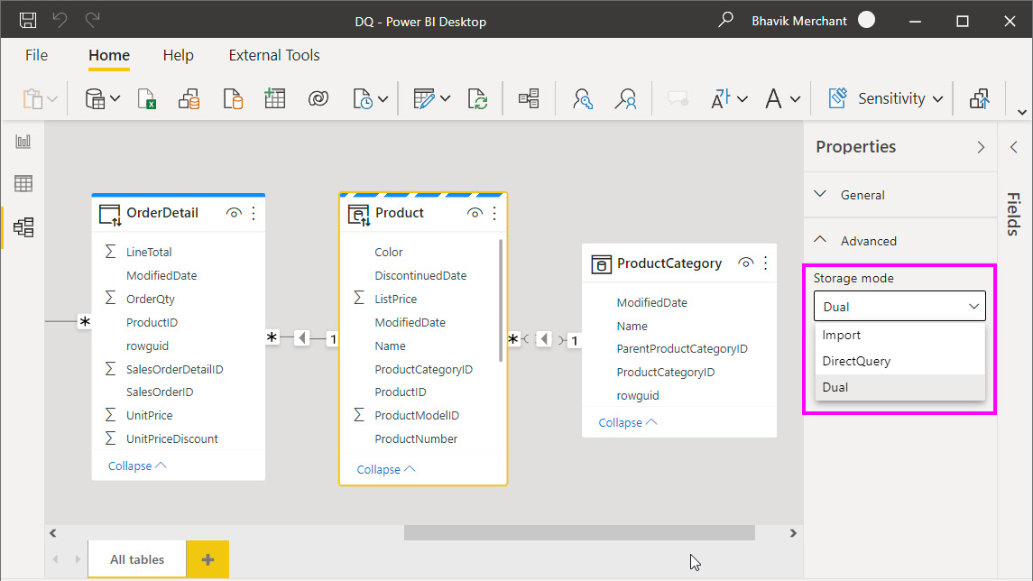
Figure 12.6 – The Storage mode setting in the Model view

There are interesting things to note in the preceding screenshot. The Storage mode dropdown offers the Import, DirectQuery, and Dual storage modes. In the model diagram view, the table header's colors and icons indicate what type of storage mode is used. With Dual mode, depending on the query's scope and granularity, Analysis Services will decide whether to use the in-memory cache or use the latest data from the data source. Let's look at these table storage modes and learn when to use them:

• DirectQuery: This is the blue header bar with the DirectQuery icon (for example, OrderDetail). Choose this mode for tables that contain very large data volumes, or where you need to fetch the latest results all the time. Power BI will never import this data during a data refresh. Typically, these would be fact tables.
• Import: This is the plain white header bar with the Import icon (for example, ProductCategory). Choose this mode for smaller or very compressible tables that need to be fast and don't change as frequently as the DirectQuery source. When you choose Import storage mode, you mustn't plan to use this table to filter or group fact tables.
• Dual: This is the banded blue and white header bar with the DirectQuery icon (for example, Product). Choose this mode for tables that act as dimensions that are used to filter or group data in the fact table – that is, DirectQuery. This means there are scenarios where the table will be queried together with fact tables at the source.

Now, let's explore how these storage modes are used by the engine in different scenarios. This will help you design and define the storage modes appropriately. This is important because it determines the type of relationship that's used, which directly impacts performance. The following are some possible query scenarios:

• Query uses Import or Dual table(s) only: This populates slicers or filters, typically on dimension tables. Such queries achieve the best performance by using the local in-memory cache.
• Query uses Dual or DirectQuery table(s) from the same source: This occurs when the query needs to relate Dual mode dimension tables to DirectQuery fact tables. It will issue one or more native queries to the DirectQuery source and can achieve relatively good performance if the source is optimized, as discussed in Chapter 3, DirectQuery Optimization. One-to-one or one-to-many relationships within the same data source are evaluated as regular relationships that perform better. A regular relationship is where the column on the "one" side contains unique values.
• Any other query: Any query that needs to resolve relationships across different data sources falls into this category. This happens when a Dual or Import mode table from source A needs to join a DirectQuery table from source B. Here, the engine uses limited relationships, which are slower. Many-to-many relationships and relationships across different data sources are limited.

Let's order relationships from best to worst performance:

• One-to-many relationships within the same source (fastest)
• Many-to-many relationships that use a bridge table and at least one bi-directional relationship
• Many-to-many relationships
• Cross-source group relationships (slowest)

Next, we will introduce aggregations and how they relate to composite models.

Leveraging aggregations

Most analytical scenarios involve aggregating data in some way. It is common to look at historical trends, exceptions, and outliers at a summary level, and then drill down to more detail as required. Let's look at an example of a logistics company tracking thousands of daily shipments to watch for delays. They are unlikely to start this analysis at the individual package level. They would more likely have some performance indicators grouped by transportation type or region. If they see unsatisfactory numbers at the summary level, they may drill down to more and more detail to narrow down the root cause. In Chapter 9, Report and Dashboard Design, we recommended designing reporting experiences like this to provide better performance and usability.

You may follow the recommended design principles and still have performance issues with very large DirectQuery datasets. Even with great optimizations, there is still a physical limit as to how fast you can process data with fixed computing resources. This is where the aggregations capability of Power BI can help. An aggregation table is a summary of another fact table but one that's always stored in Import mode in memory. As such, aggregation tables must be reloaded during data refresh.

We will build on the example shown in Figure 12.6 to illustrate this. We want to add aggregations to the OrderDetail table to avoid generating an external DirectQuery. Suppose our requirements have determined that many reports aggregate total sales at the product level. We can achieve better performance by adding an aggregation table. We will add a table in Import mode called Agg_SalesByProduct that's defined by the following SQL expression:

SELECT

ProductID,

sum(sod.LineTotal) as TotalSales,

sum(sod.OrderQty) as TotalQuantity

FROM

[SalesLT].[SalesOrderDetail] sod

GROUP BY ProductID

Once the aggregation table exists, we need to tell Power BI how to use it. Right-click the OrderDetail table in the model view, select the Manage aggregations option, and configure the aggregations, as shown in the following screenshot:

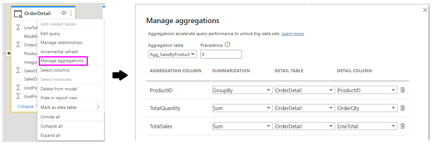
Figure 12.7 – Configuring the aggregations for OrderDetail

There are a few things to note in the previous screenshot. First, we had to tell Power BI which table we wanted to use as an aggregate for OrderDetail. We also had to map the columns and identify what type of summarization was used. There is also the option to select precedence because you can have multiple aggregation tables at different granularities. Precedence will determine which table is used first when the result can be served by more than one aggregation table. Once the aggregations have been configured, the final step is to create the relationship between the aggregation table and the Product dimension, as shown in the following screenshot:

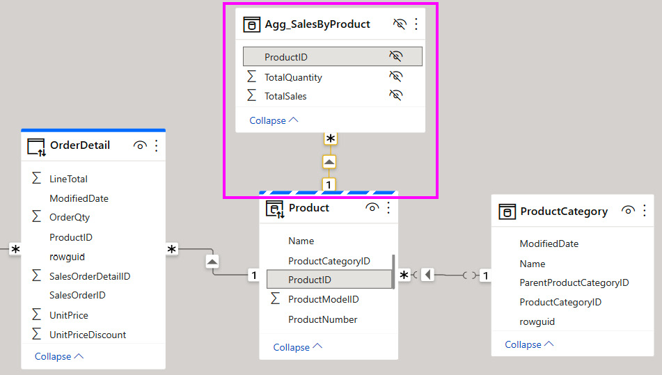
Figure 12.8 – The Import mode Agg_SalesByProduct table related to the Dual mode Product table

In the preceding screenshot, notice that the aggregation table and its columns are all hidden in the Power BI dataset. Power BI will do this by default since we do not want to confuse users. We can hide aggregation tables and rely on the engine to pick the correct tables internally.

Note

The example shown in the preceding screenshot demonstrates aggregations based on relationships. We are relying on a relationship so that the values from the Product table could filter OrderDetails. When we added the aggregation table, we needed to create this relationship.

In typical big data systems based on Hadoop data is often stored in wide denormalized tables to avoid expensive joins at query time. We can still use aggregations in Power BI for such a scenario, but we wouldn't need to create any relationships.

Next, we'll learn how to identify when and which aggregations are used with DAX Studio. We will begin by constructing three table visuals showing different sales groupings. You can see these in the sample file on the Aggs Comparison report page:

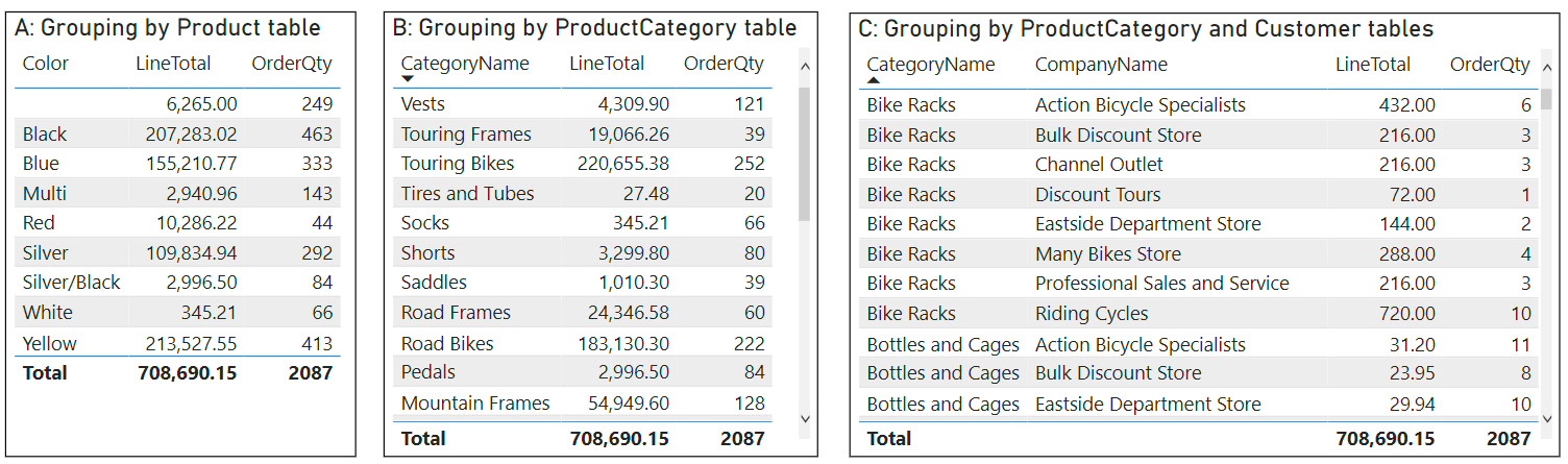
Figure 12.9 – Different sales groupings to test aggregations

The visual titles in the preceding screenshot refer to the tables in the sample, which are shown in Figure 12.8. We constructed the visuals in Figure 12.9 at different granularities, using different grouping tables, to see how the queries behave. We used DAX Studio to capture the output and found the following:

• A: Grouping by Product table: The query was completely satisfied through Import tables. Only one storage engine query was needed. Note how DAX Studio provides information on the RewriteAttempted event subclass, which means the engine recognized that aggregations were present and tried to use them. You can click on the event to get the detail on the right-hand side, confirming which aggregation table was used:

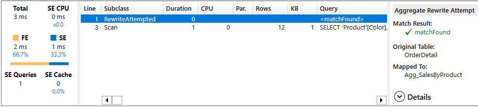
Figure 12.10 – Query performance information for visual A

• B: Grouping by ProductCategory table: Again, the query was completely satisfied through Import tables. What is great here is that even though ProductCategory is not directly related to the aggregation table, the engine does use it, leveraging the Product table as a bridge. This has allowed us to avoid an external query for a scenario that we did not originally plan for:

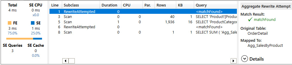
Figure 12.11 – Query performance information for visual B

• C: Grouping by Product and Customer table: This time, the query tried to use aggregation for a customer but was unable to since we did not define our aggregation at the customer granularity level. The engine did use an external query, which is proven by the SQL event subclass. However, it was still able to use the aggregation table later:

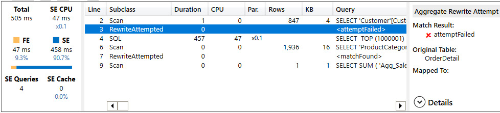
Figure 12.12 – Query performance information for visual C

The previous examples demonstrate how aggregations are used, but we have not compared the same query with and without aggregations yet. To test this, we can simply delete the aggregation table and profile the same visuals in DAX Studio, with the following total query durations:

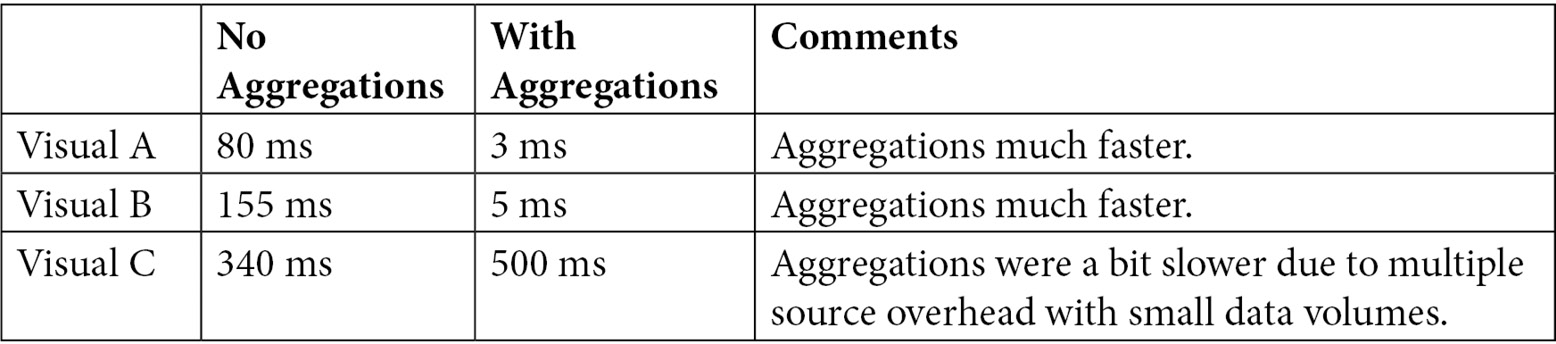
Figure 12.13 – Performance comparison of different visual groupings with aggregations

In our example, designing and managing aggregations would be simple. In the real world, it can be difficult to predict the complexity, volume, and frequency of the queries that will be generated. This makes it hard to design aggregations beforehand. Microsoft has considered this problem and has released automatic aggregations as an enhancement to user-defined aggregations. With automatic aggregations, the system uses machine learning to maintain aggregations automatically based on user behavior. This can greatly simplify aggregation management if you can use it.

Note

Automatic aggregations are currently only available to the Power BI Premium and Embedded capacities. The feature is in preview and subject to change, so we won't provide further details. Check out the relevant documentation to learn more: https://docs.microsoft.com/power-bi/admin/aggregations-auto.

Finally, let's touch on Azure Synapse and Data Lake. These are first-party technologies from Microsoft that you may wish to consider for external data storage in big data scenarios that need DirectQuery.

Scaling with Azure Synapse and Azure Data Lake

Many data analytics platforms are based on a symmetric multi-processing (SMP) design. This involves a single computer system with one instance of an operating system that has multiple processors that work with shared memory, input, and output devices. This is just like any desktop computer or laptop we use today and extends to many server technologies too. An alternative paradigm is massively parallel processing (MPP). This involves a grid or cluster of computers, each with a processor, operating system, and memory. Each machine is referred to as a node.

In practical terms, consider computing a sum across 100 billion rows of data. With SMP, a single computer would need to do all the work. With MPP, you could logically allocate 10 groups of 10 billion rows each to a dedicated computer, have each machine calculate the sum of its group in parallel, and then add up the sums. If we wanted the results faster, we could spread the load further with more parallelism, such as by having 50 machines handle about 2 billion rows each. Even with communications and synchronization overhead, the latter approach will be much faster.

Big data systems such as Hadoop, Apache Spark, and Azure Synapse use the MPP architecture because parallel operations can process data much faster. MPP also gives us the ability to both scale up (bigger machines) and scale out (more machines). With SMP, only the former is possible until you reach a physical limit regarding how large a machine you can provision.

The increasing rate of data ingestion from modern global applications such as IoT systems creates an upstream problem when we think about data analysis. BI applications typically use cleaned and modeled data, which requires modeling and transformation beforehand. This works fine for typical business applications. However, with big data, such as a stream of sensor data or web app user tracking, it is impractical to store raw data in a traditional database due to the sheer volume. Hence, many big data systems use files (specially optimized, such as Parquet) that store denormalized tables. They perform Extract-Load-Transform (ELT) instead of the typical Extract-Transform-Load (ETL) as we can do in Power Query. With ELT, raw data is shaped on the fly in parallel.

Now, let's relate these concepts to the data warehouse architecture and the Azure offerings.

The modern data warehouse architecture

We can combine traditional ETL style analytics with ELT and big data analytics using a hybrid data warehouse architecture based on a data lake. A data lake can be described as a landing area for raw data. Data in the lake is not typically accessed directly by business users.

Once data is in the lake, it can be used in different ways, depending on the purpose. For example, data scientists may want to analyze raw data and create subsets for machine learning models. On the other hand, business analytics team members might regularly transform and load some data into structured storage systems such as SQL Server. The following diagram shows a highly simplified view of Azure components that could make up a modern data warehouse:

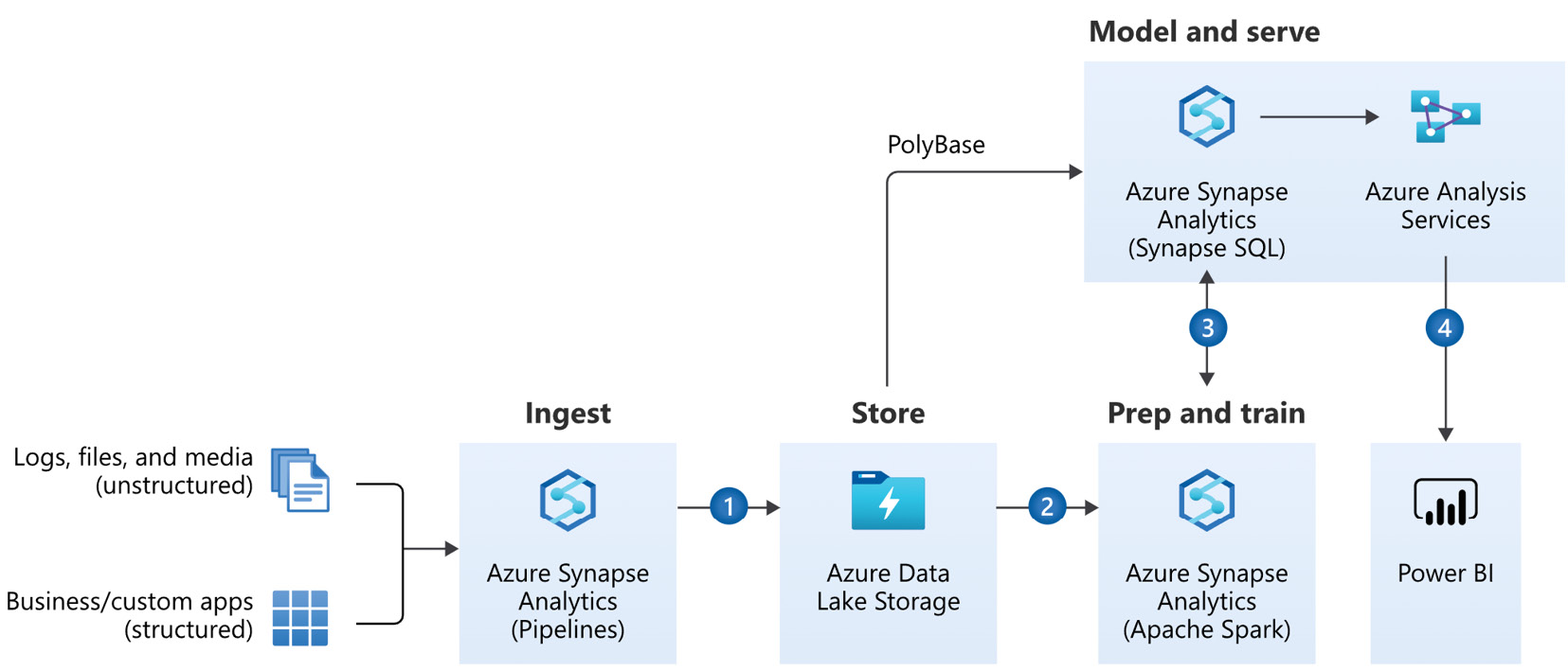
Figure 12.14 – A modern data warehouse architecture (image credit: Microsoft)

The numbered steps in the preceding diagram indicate typical activities:

1. Store all types of raw data in Azure Data Lake Storage using Azure Synapse Analytics pipelines.
2. Leverage Synapse Analytics to clean up data.
3. Store clean, structured data in Synapse SQL and enrich it in Azure Analysis Services.
4. Build reporting experiences over Synapse and Azure Analysis Services using Power BI.

   Note

   The steps in the preceding diagram are ordered, and the diagram only shows connections between some components. This represents production-style data paths and is only to aid learning. In a modern enterprise, it is realistic to skip some steps or connect different technologies, depending on the scenario and user's skill level. For example, a data engineer may connect Power BI directly to ADLS to explore data format and quality. Other Azure services complement this architecture, which haven't been shown.

Now, let's take a closer look at some technologies that help with data scaling.

Azure Data Lake Storage

Azure Data Lake Storage (ADLS) is a modern data store that's designed for big data scenarios. It provides limitless storage and is compatible with non-proprietary technologies such as Hadoop Distributed File System (HDFS), which is a core requirement for many Hadoop-based systems. Note that the current version is referred to by Microsoft as ADLS Gen2, indicating that we are in the second generation offering. While the original data lake technology is still available, we recommend using Gen2 as it offers better performance and functionality. Platforms such as Synapse will only work on Gen2. Synapse services are optimized to work with data in parallel over ADLS.

Azure Synapse analytics

Azure Synapse is an analytics platform that contains different services that address the special needs of different stages of data analytics. It was previously called SQL Server Data Warehouse, and at the time, the focus was to provide a distributed version of SQL Server to handle multi-terabyte and larger data volumes. Since then, it has been rebranded and grown into a complete suite that offers the following services and capabilities:

• Synapse Studio: A web-based environment that serves multiple personas. People can ingest, transform, explore, and visualize data here.
• Power BI integration: You can link Power BI workspaces to your Synapse workspace in Synapse Studio. Then, you can analyze data hosted in Synapse services using Power BI within Synapse Studio.
• Notebook integration: Synapse Studio supports Python notebooks for interactive data exploration and documentation.
• Serverless and dedicated SQL pools: These offer structured SQL Server storage in the cloud. A serverless pool needs little configuration and management – you do not need to provision a server, the service auto-scales, and you pay per query. A dedicated pool must be configured beforehand and is billed constantly over time. Dedicated pools can be paused and scaled up or down. These options provide a balance between costs and management overhead.
• Serverless and dedicated Spark pools: Apache Spark is a very popular open source big data platform. It is an in-memory technology and offers a SQL interface over data. It also offers integrated data science capabilities. Synapse integrates with Spark pools directly, allowing analysts to run Spark Jobs from Synapse Studio.
• Data flows: These provide visually designed data transformation logic to clean and shape data using the power of processing pools.
• Data pipelines: Allows users to orchestrate and monitor data transformation jobs.

There are many options and variations within the modern data warehouse architecture. Unfortunately, it is beyond the scope of this book to cover these. Microsoft offers multiple reference architectures to deal with analytics problems, ranging from business data warehousing to near-real-time predictive analytics on streaming data. Therefore, we recommend checking out the Microsoft Azure Architecture site to learn about which Azure services can be used for varying analytics needs: https://docs.microsoft.com/azure/architecture/browse/?azure_categories=analytics.

Now that we have provided an introduction to the Azure technologies we can use to deal with data at a high scale, let's summarize what we've learned in this chapter.

Summary

In this chapter, we learned how to deal with exceptionally large volumes of data. The first use case was where we had Power BI datasets growing beyond the 1 GB storage limit that's available to Power BI Pro users in the Shared capacity. In such cases, we recommended considering Power BI Premium. The dataset limit in Premium is 10 GB. With the large dataset storage format enabled, we learned that datasets could grow well beyond this size. Technically, we can use all the available memory on the capacity, which is 400 GB on a Premium P5 capacity. Larger Premium capacities also have higher concurrency limits, which can give us better refresh and query performance.

Then, we looked at a case where the scale problem comes from concurrent users and learned why this can put pressure on memory and CPU resources. We introduced AAS as a solution to this problem due to its ability to leverage QSO. We also recommended using partitions on Premium and AAS to speed up refreshes on large tables. We advised you to carefully consider the features and roadmap of Premium versus AAS as there are currently differences.

After that, we looked at improving DirectQuery performance with composite models, a feature that lets you combine Import and DirectQuery sources into the same Power BI dataset. We saw how Power BI controls storage mode at the table level and that we can configure individual tables as Import, DirectQuery, or Dual. The Dual mode tables will Import data and store it in local memory and allow DirectQuery when needed. We showed you when to use these storage modes and how Analysis Services will choose the best option, depending on the scenario.

Next, we looked at aggregations, a complementary feature to composite models. Microsoft designed aggregations around the premise that data from large fact tables is often summarized. Even with good optimizations in a DirectQuery source, summaries over tens of millions to billions of rows can still take time. The problem is worse when we have high user concurrency. An aggregation table in Power BI allows us to define grouped subsets of fact tables, which Analysis Services can use as an alternative to a slow down DirectQuery. You can achieve huge performance gains when aggregate tables are in Import mode.

Finally, we looked at other technologies from Microsoft that can deal with big data problems. We learned that it is not practical to ingest and transform certain types of data due to their sheer speed and volume. Hence, big data systems tend to use the MPP architecture and rely on ELT paradigms to shape data on demand for different purposes. In the modern data warehouse, all raw data is stored in a central data lake first. Different technologies sit over the lake and perform exploration, ETL, or ELT as suits the use case. We introduced Azure Data Lake Storage and Azure Synapse Analytics as the primary technologies you can use to implement a modern data warehouse.

In the next chapter, we will focus on the Power BI Premium and Embedded capacities. Here, Microsoft provides you with settings and controls where there are additional performance considerations.

Further reading

Note that just like Power BI, every area of Synapse benefits from specific performance tuning guidance. The following are some references to the relevant performance guidance material:

• Serverless SQL pool best practices: https://docs.microsoft.com/azure/synapse-analytics/sql/best-practices-serverless-sql-pool
• Dedicated SQL pool best practices: https://docs.microsoft.com/azure/synapse-analytics/sql/best-practices-dedicated-sql-pool
• Azure Advisor recommendations for dedicated SQL pools: https://docs.microsoft.com/azure/synapse-analytics/sql-data-warehouse/sql-data-warehouse-concept-recommendations
• Materialized view optimization: https://docs.microsoft.com/azure/synapse-analytics/sql/develop-materialized-view-performance-tuning
• Clustered index optimization: https://docs.microsoft.com/azure/synapse-analytics/sql-data-warehouse/performance-tuning-ordered-cci
• Result set cache optimization: https://docs.microsoft.com/azure/synapse-analytics/sql-data-warehouse/performance-tuning-result-set-caching
• Optimizing Synapse query performance tutorial: https://docs.microsoft.com/learn/modules/optimize-data-warehouse-query-performance-azure-synapse-analytics
• Tuning Synapse data flows: https://docs.microsoft.com/azure/data-factory/concepts-data-flow-performance?context=/azure/synapse-analytics/context/context