6

Inventor Assembly Fundamentals – Constraints, Joints, and BOMS

The Inventor Assembly environment is used to combine multiple part files, subassemblies, and components to create a bottom-down assembly that communicates how all individual parts are combined and interface with each other. The assembly environment can also be used to edit parts and model subsequent parts if required.

The Inventor Assembly environment is instrumental in ensuring tolerance, fit, overall function, and the overall working of a completed product or subassembly. In previous chapters, we used the assembly environment, but in this chapter, we will cover the best practices for assembling parts, managing a Bill of Materials (BOM), and how you can duplicate and replace components within an assembly.

In this chapter, we will learn the following:

• Constraining components in assemblies – the best practices
• Applying joints in assemblies
• Applying and driving Motion constraints
• Duplicating and replacing components in an assembly
• Creating and configuring a BOM
• Detailing and customizing a BOM in a drawing file

Technical requirements

To complete this chapter, you will need access to the practice files in the Chapter 6 folder within the Inventor Cookbook 2023 folder.

Constraining components in assemblies – the best practices

In this recipe, you will use constraints and assemble a brake assembly from multiple Inventor parts and subassemblies. In doing this, we will cover best practices with the Constraint tool.

You may have noticed that within Inventor, there are two distinct methods of combining parts together in an assembly – Joints and Constraints. Both can be used independently or combined together to achieve the desired design intent.

Both assembly constraints and assembly joints are used to create relationships between components that determine a component’s location and the allowable movement.

The Constrain and Assemble commands are methods of positioning components by gradually eliminating degrees of freedom (DOF). This is a legacy feature within Inventor and predates the introduction of assembly joints.

Inventor joints are used to simplify the complexity of component relationships. With a Joint, you not only define the position of a component but also fully define the allowable motion.

In the following recipe, we will just focus on constraints.

Getting ready

To begin this recipe, you will need to create a New Metric (mm) Standard Assembly.iam file and have this open in Inventor.

How to do it…

To begin, ensure that you have a New Metric (mm) Standard.iam file open in Inventor. We will start by placing one component at a time and adding constraints to fully define the assembly. The completed assembly you will create with constraints is shown in Figure 6.1:

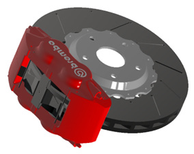
Figure 6.1: The completed brake assembly

To begin, we will first place the component by following these steps:

1. Within your newly created assembly file, navigate to the Assemble tab and select Place Component.
2. Navigate to the Chapter 6 folder | the Brake folder, and select DRIVER_ BRAKE_ROTOR.ipt. Select Open.
3. The component now opens in your new assembly and is fixed on your cursor. Instead of left-clicking to place the new component, we first need to ground it. This is important, as this will fix the first component to the origin of the assembly file. Without this, the component would be undefined, and we would have difficulty assembling the rest of the components to it. A grounding of components is only usually required when the first component of your assembly is placed.

Right-click anywhere in the Graphics Window, and select Place Grounded at Origin from the Graphics Window options that appear.

4. The first component is now placed, and we can now proceed to add another component. Select Place from the Assemble tab.
5. Navigate to the Chapter 6 folder | the Brake folder, select BRAKE_HUB.ipt, and then select Open.
6. Left-click anywhere to place the BRAKE_HUB file into the assembly. Note that the component is floating in the Graphics Window and is not fixed. If you click and drag the component, you will see that it moves freely as no DOF have been locked. We will now use the Assembly constraint to apply DOF and fix the component in relation to the DRIVER_BRAKE_ROTOR file, as desired.
7. Select Constrain from the Assemble tab. We are now able to select faces, edges, and planes to constrain the components together. We can also define the Mate type we want to place. Leave the defaults in the Mate Constrain window as they are; we will be using standard Mates for now.

Before assembling a product in Inventor, it is a good idea to know how they go together first. Having a good understanding of the model and parts will enable you to assemble them more efficiently and allow you to use the minimal number of Mates required. Always look for symmetry in the model and shared centerlines or planes with the components!

With Constrain selected, select the bottom face of BRAKE_HUB as the first reference, as shown in Figure 6.2:

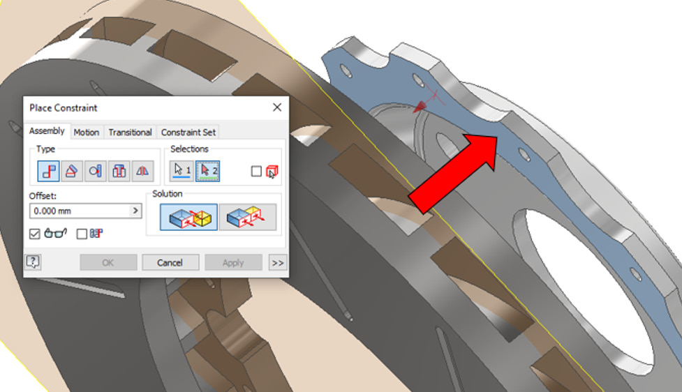
Figure 6.2: First face selected of BRAKE_HUB with the Mate Constrain tool

8. Rotate the model and select the face shown in Figure 6.3 of DRIVER_BRAKE_ROTOR to act as the second reference for this Mate. This way, we are communicating to Inventor that we want these two faces to be in contact with each other. Then, select Apply:

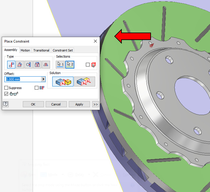
Figure 6.3: The second reference for the Mate

9. The first Mate has been created, although the component is not fully defined as it can still be moved and has DOF. To see what DOF are remaining, you can select the Degrees of Freedom button at the top left of the View tab within an assembly. Selecting this will reveal to what degrees the components can move.

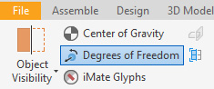
Figure 6.4: Degrees of Freedom

Another option is to grab and move the component and see how it can be manipulated with a mouse drag.

10. We will now define the component further with more mates. In the model browser to the left of the screen, note that the Relationships folder has become populated with 1 Mate. This is the Mate we created in Step 8. At any time, you can right-click on the Mate in the model browser, edit the parameters, and delete or even rename the Mate.

In the Assemble tab, select Constrain.

11. Navigate to the center of BRAKE_HUB and select the geometry shown in Figure 6.5, and then the centerline of this component should be highlighted.

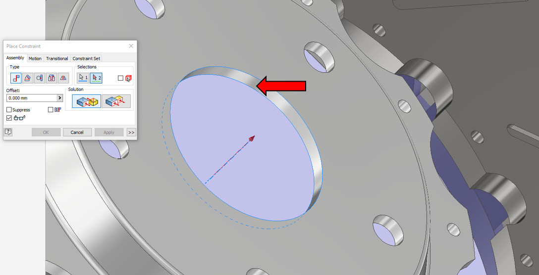
Figure 6.5: The first reference for Mate 2 to select

We will now use the Mate to align the components on a shared centerline.

12. For the second reference of this Mate, rotate to the other side of the model, and select the internal diameter shown in Figure 6.6. Select Apply to complete the Mate.

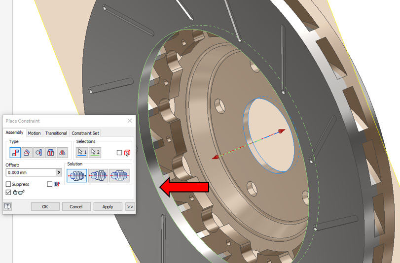
Figure 6.6: Internal diameter to select to complete Mate 2 and align the components on a common centerline

13. Although the two components are flush together and aligned at the center, BRAKE_HUB needs to be aligned with DRIVER_BRAKE_ROTOR.

Select the constraint, and then select the internal diameter of one of the small holes on BRAKE_HUB as the first reference.

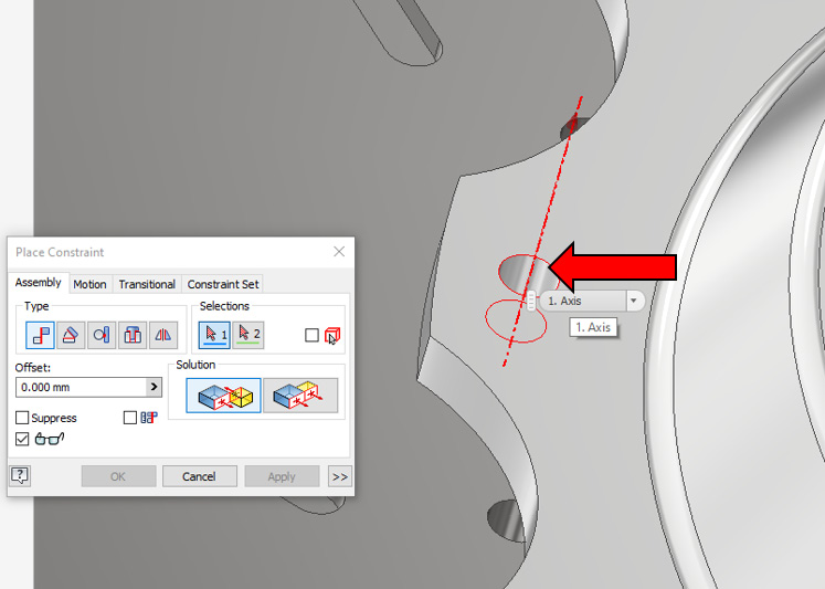
Figure 6.7: The Mate constraint on the internal diameter of small holes in BRAKE_HUB

14. For the second reference, select the corresponding hole on DRIVER_BRAKE_ROTOR, and then select Apply.

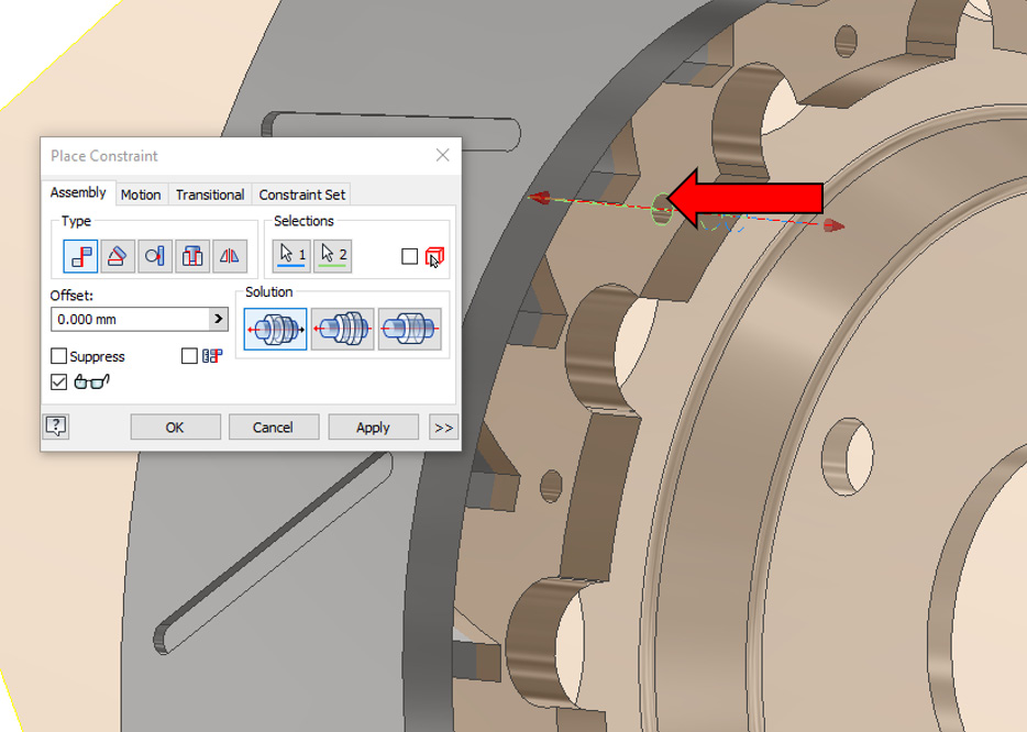
Figure 6.8: The second reference to select for the Mate Constraint

This will fully define the two components so that they are placed correctly and have no more DOF. It is common practice to apply more than one mate to a component to achieve this.

15. Select Place, and browse for CALIPER.ipt in the Chapter 6 folder. Select Open. Left-click to place the part in your assembly, and then hit Esc to exit the placing of components.
16. Select Constrain, and select the face of CALIPER, as shown in Figure 6.9, as the first reference:

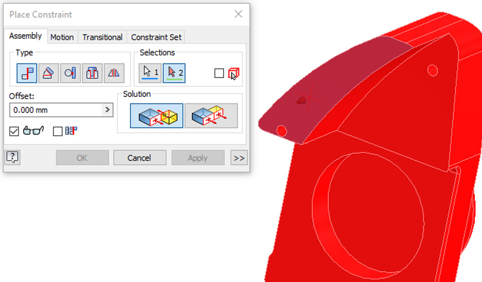
Figure 6.9: The first reference of CALIPER to select

17. Select the work plane of DRIVER_BRAKE_ROTOR as the second reference. As we have an internal central plane, we can align our part to this. Then, select Apply:

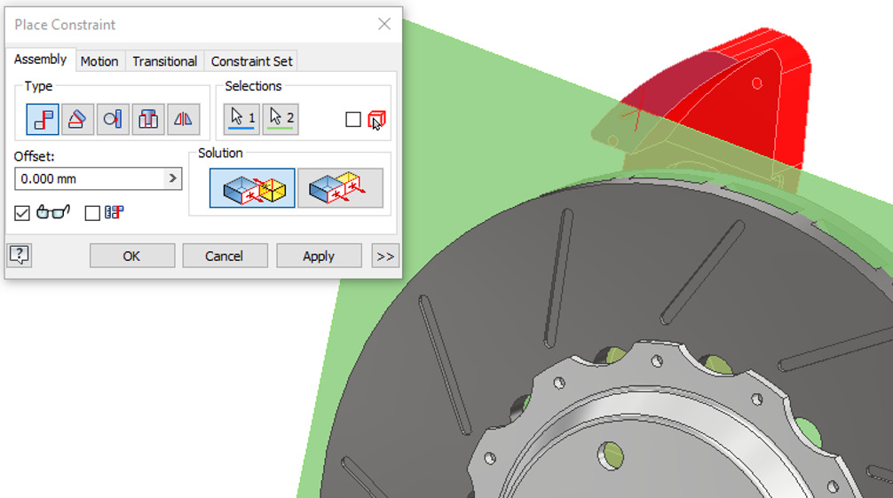
Figure 6.10: The second reference to select of CALIPER

18. Select Place and browse for RETAINER_PIN.ipt. Select Open and left-click anywhere to place in the assembly.
19. Select Constrain. Within the Model Browser on the left of the screen, expand the CALIPER part by selecting +. Expand the Origin folder by selecting +. Then, select YZ Plane as the first reference:

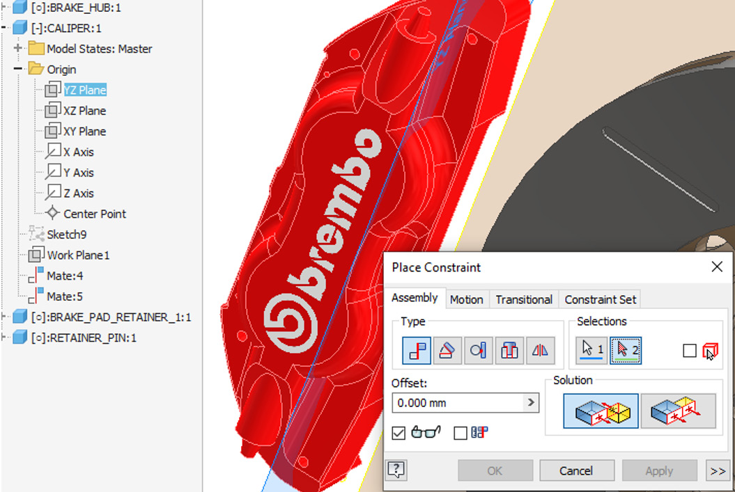
Figure 6.11: YZ Plane of Caliper selected as the first reference

20. Within the model browser on the left of the screen, expand the DRIVER__BRAKE_ROTOR part by selecting +. Expand the Origin Folder by selecting +. Then, select YZ Plane as the first reference.
21. In the offset area of the Place Constraint menu, type -130mm and select Apply:

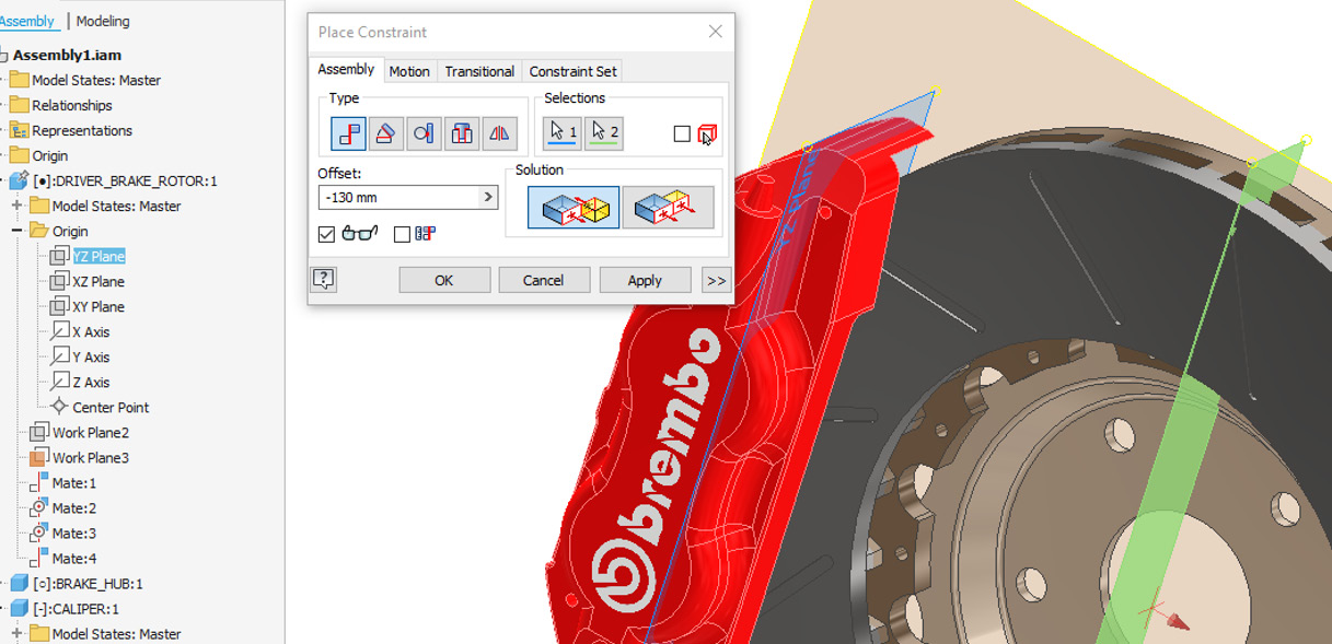
Figure 6.12: YZ planes of each component mated with a -130mm offset applied

There is still one more DOF on the CALIPER. Select Constrain, and place a Mate Constraint between XZ Plane of CALIPER and XZ Plane of DRIVER__BRAKE_ROTOR.

22. Select Place and browse for BRAKE_PISTON.ipt. Select Open and left-click anywhere to place in the assembly.
23. Select Constrain, and then select Insert Mate Constraint, followed by the geometry on BRAKE_PISTON, as shown in Figure 6.13, as the first reference.

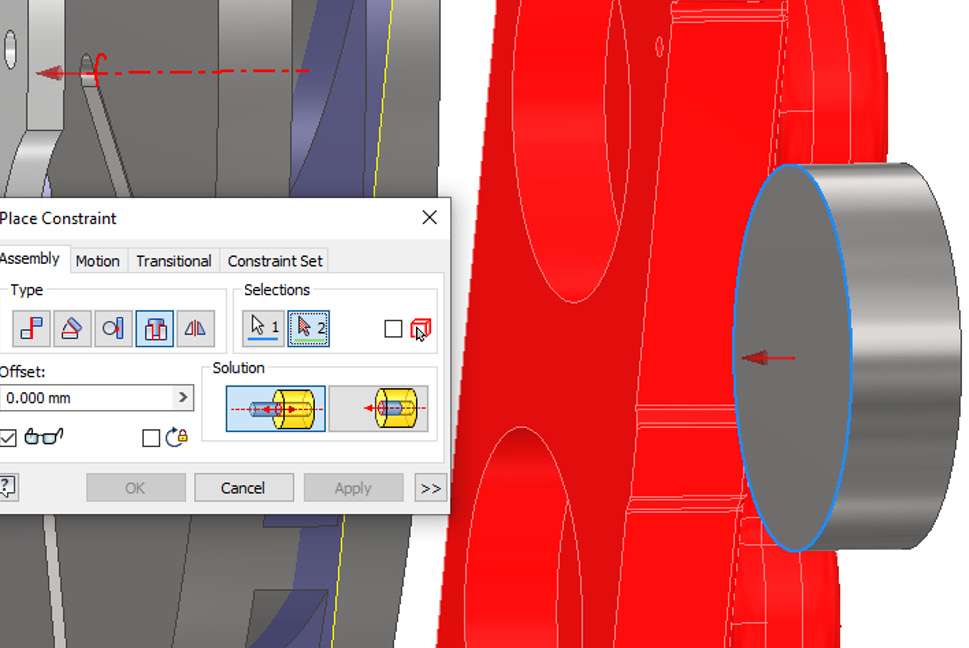
Figure 6.13: The first reference of BRAKE_PISTON to select

24. Select the internal geometry of CALIPER, as shown in Figure 6.14, as the second reference, and then select Apply:

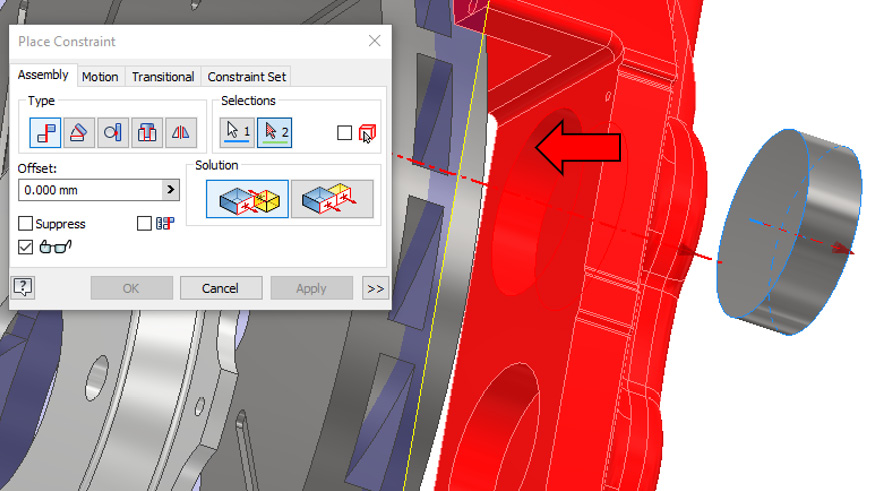
Figure 6.14: The second reference of CALIPER to select

25. Repeat steps 23 to 24 to add another instance of BRAKE_PISTON and Mate it into position within the assembly. Once this is done, there should be two instances of BRAKE_PISTON on CALIPER, as shown in Figure 6.15:

Figure 6.15: Two instances of BRAKE_PISTON defined and placed in the assembly

26. Select Place and browse for BRAKE_PAD.ipt. Select Open and left-click anywhere to place in the assembly.
27. Select Constrain and select the face of BRAKE_PAD shown in Figure 6.16 as the first reference:

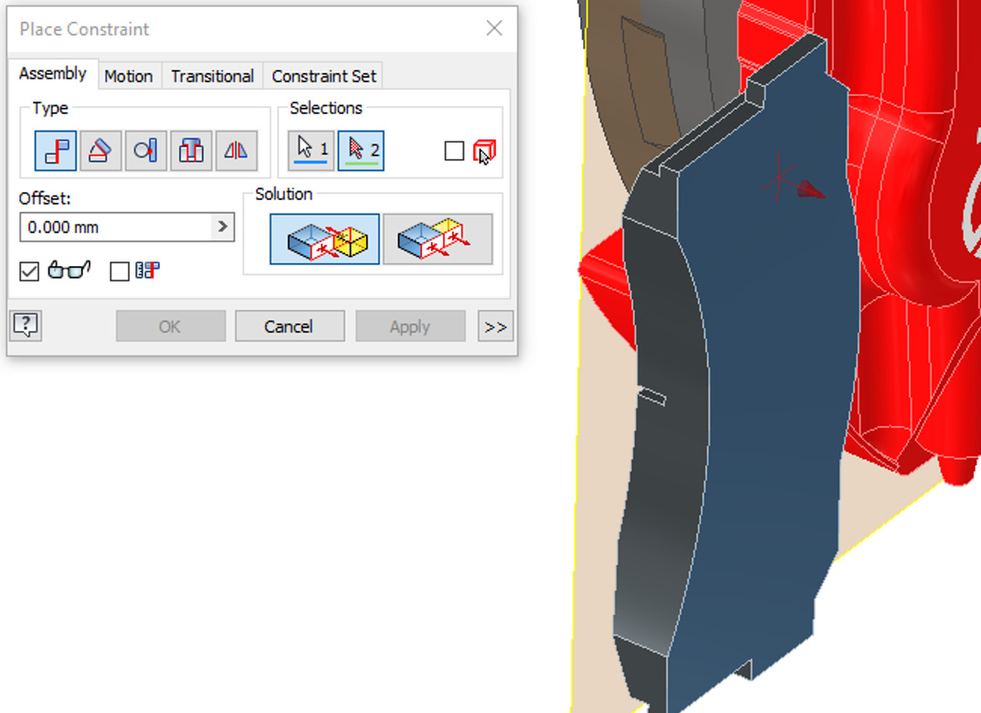
Figure 6.16: The first reference of BRAKE_PAD to select

28. For the second reference, select the top face of BRAKE_PISTON, as shown in Figure 6.17:

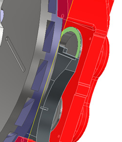
Figure 6.17: The second reference selected

29. Click and drag BRAKE_PAD away from the assembly. The previous mate we created in step 28 will still be active. Pulling the component away while not fully defined allows us to see all available faces to select for further mates. Another option would be to change the visibility of components, or to adjust the visual style of the model:

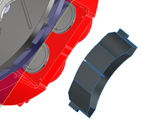
Figure 6.18: BRAKE_PAD manually moved from the assembly

30. Select Constrain and proceed to select the geometry shown in Figure 6.19 as the first reference:

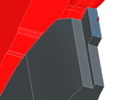
Figure 6.19: The top face of BRAKE_PAD selected as the first reference

31. Figure 6.20 shows the second reference to select. Select Apply to complete:

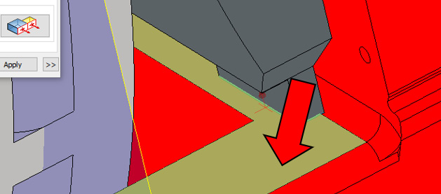
Figure 6.20: The second reference of CALIPER to select

32. Select the geometry shown in Figure 6.21 to align and eliminate all final DOF on BRAKE_PAD. This is the top face of the pad and the edge of CALIPER, as shown in Figure 6.21. Then, select Apply:

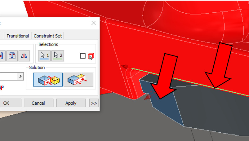
Figure 6.21: The final Mate Constraint to create on RETAINER_PIN

33. Select Constrain | Insert Constraint, and then the reference shown in Figure 6.22 of RETAINER_PIN: 1:

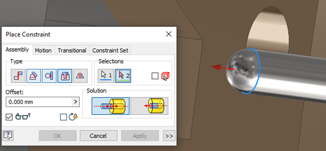
Figure 6.22: The first Insert Mate reference on RETAINER_PIN 1

34. For the second reference, select this geometry on CALIPER. Then, select Aligned as the Solution option. The result resembles Figure 6.23. Select Apply to complete.

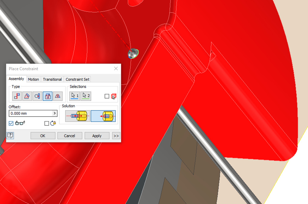
Figure 6.23: The final Insert Mate reference to make on CALIPER with Aligned selected as the Solution option

35. Repeat steps 33 to 34 to place and constrain another instance of the RETAINER_PIN in the correct position, as shown in Figure 6.24:

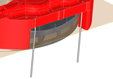
Figure 6.24: The second instance of RETAINER_PIN constrained in position

36. Select Place and browse for BRAKE_PAD_RETAINER_1.ipt. Select Open and left-click anywhere to place in the assembly.
37. Select Constrain in the model browser on the left of the screen, expand + next to DRIVER_BRAKE_ROTOR, and then expand + next to BRAKE_PAD_RETAINER. We will now work to align this component centrally to the model, as is the design intent.
38. Select + and expand the Origin folder of DRIVER_BRAKE_ROTOR. Select Work Plane 3 as the first reference for this Mate.
39. Select + and expand the Origin folder of BRAKE_PAD_RETAINER_1. Select YZ Plane as the second reference of this Mate. Then, select Apply to complete.

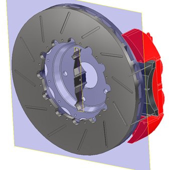
Figure 6.25: The BRAKE_PAD_RETAINER_1. YZ plane mated to WorkPlane3 of DRIVER_BRAKE_ROTOR

40. Select Mate Constrain, and create a Mate between BRAKE_PAD_RETAINER_1 and RETAINER_PIN, as shown in Figure 6.26. Select Apply to complete.

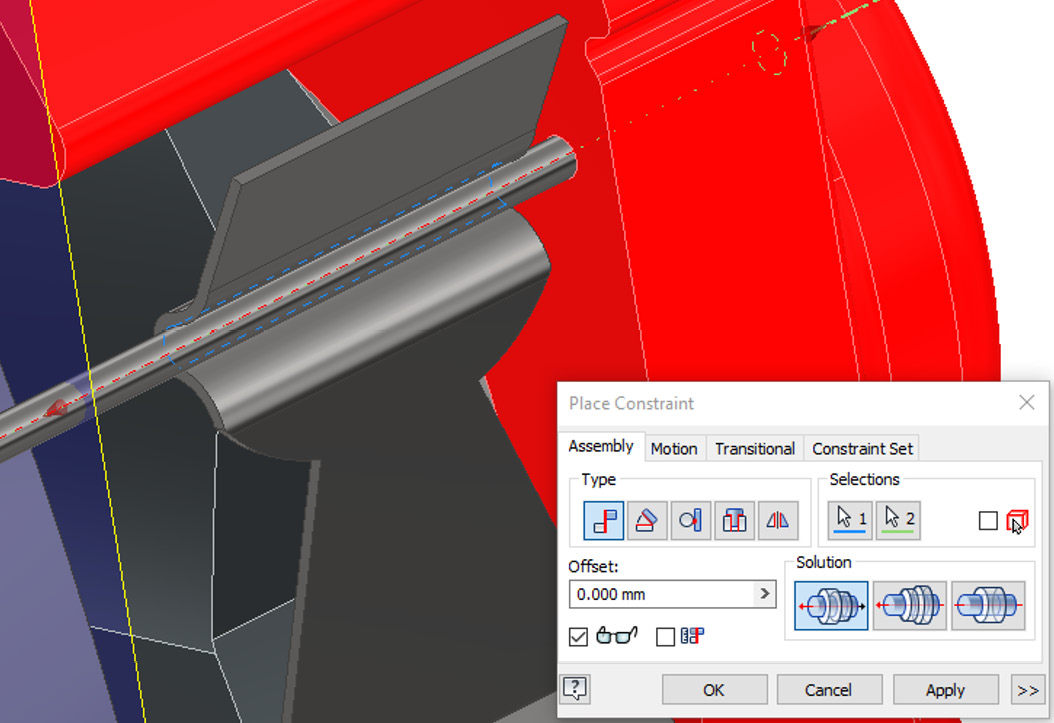
Figure 6.26: The Mate constraint between BRAKE_PAD_RETAINER_1 and RETAINER_PIN

41. Select Constrain, and then select Angle as the Type option. Select the faces shown in Figure 6.27 as the reference. Then, select Directed Angle as the Solution option for the Angle Mate constraint. Leave the Angle value as 0. Select Apply to complete:

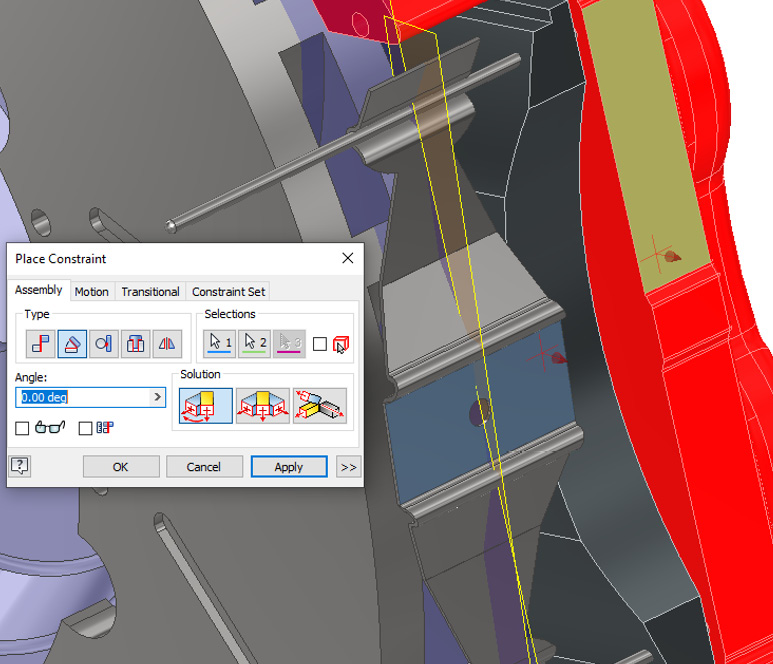
Figure 6.27: The Angle constraint applied to BRAKE_PAD_RETAINER_1 and CALIPER

42. We have now assembled half of CALIPER. Next, rather than placing second instances of all the components again and reapplying the same mates, we will instead look to mirror the components and mates around a central work plane. Always look for symmetry in instances when constraining components, as the use of the Mirror command improves efficiencies dramatically.

Within the Assemble tab, navigate to the Pattern tools and select Mirror.

43. In the Mirror command, within the Graphics Window, select the components, as shown in Figure 6.28. These are the components that will be mirrored.

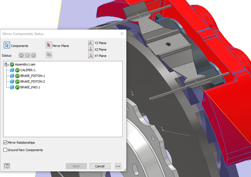
Figure 6.28: Components we need to mirror are selected

44. Select the green icon within the Mirror Components: Status window, next to Assembly1.iam. This will change all the mirror green icons of the selected components to a yellow + so that they are reused instead.

Mirror, which was the default, would create mirrored copies of the parts with a MIR suffix. Selecting Reuse makes Inventor reuse the component and create a second instance of this component.

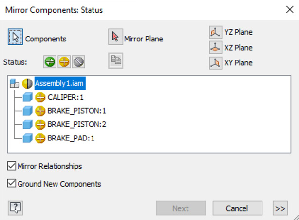
Figure 6.29: The reused components selected

45. Ensure that Mirror Relationships and Ground New Components are selected. Then, select the red arrow next to Mirror Plane.
46. Select Work Plane3 as the mirror plane from DRIVER_BRAKE_ROTOR. A preview is created once this is done.
47. Select Next, followed by OK, to complete the Mirror operation.
48. Select Place and browse for BRAKE_PAD_RETAINER_2.ipt. Select Open and left-click anywhere to place in the assembly.
49. Select Constrain and select the face of BRAKE_PAD_RETAINER_2 as the first reference, as shown in Figure 6.30:

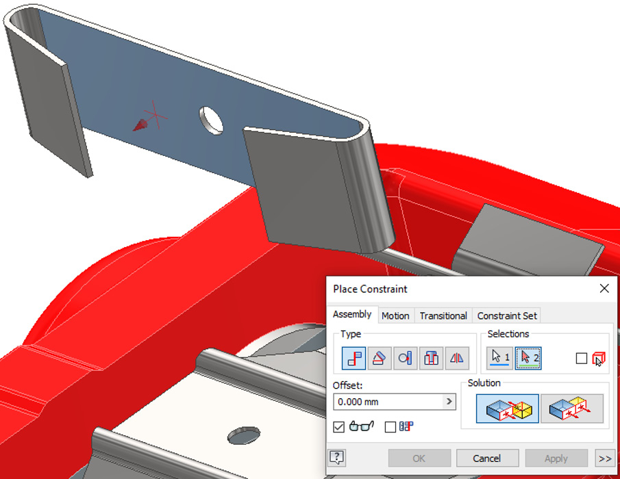
Figure 6.30: The first reference to select for the Mate constraint of BRAKE_PAD_RETAINER_2

50. For the second reference, select the face of BRAKE_PAD_RETAINER_2, as shown in Figure 6.31, and then select Apply:

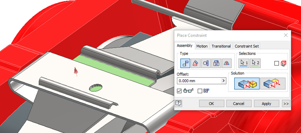
Figure 6.31: The second reference to select for the Mate constraint of BRAKE_PAD_RETAINER_2

51. Create a new Mate constraint between YZ Plane of BRAKE_PAD_RETAINER_1 and BRAKE_PAD_RETAINER_2.
52. Create a final Mate between the two central holes to align them:

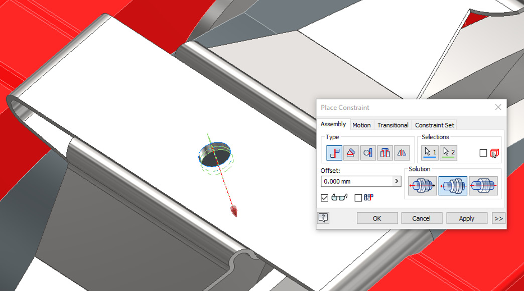
Figure 6.32: Aligned holes of the two components

The assembly of the brake caliper is now complete. You have successfully imported instances of separate parts into an assembly and used various constraints to assemble the completed design. The application of the Mirror command has meant we only had to spend time assembling half of the model.

Applying Joints in assemblies

The Joint command is an alternative to the Constrain command that enables you to define an assembly, with a specified and allowable amount of movement. Joints are selected from a pre-defined list of possible connections and then placed directly onto a model, as constraints are.

The process for assigning a joint to a component is as follows:

1. First, the Joint command is selected.
2. The Joint type is then selected.
3. References on the component are selected.
4. The limits of movement are defined.
5. The Joint is complete. Once completed, Joints can be flexed or edited to suit.

The types of Joints that you have within Inventor are as follows:

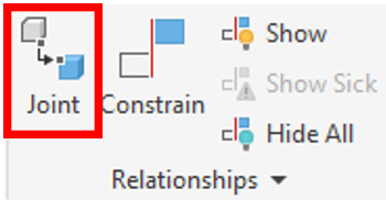
Figure 6.33: The Joint command in the assembly environment

• Automatic: This is the default Joint that is selected upon launching the command. This type of Joint enables Inventor to assume the type of Joint connection to create, based on the references picked. If the wrong one is selected, you can edit and change the type if required.
• Rigid: This Joint removes all DOF and “fixes” the component in place. In this respect, it is similar to a Mate constraint.
• Rotational: This Joint allows for rotation about an axis.
• Slider: This Joint allows for translational movement along an axis.
• Cylindrical: This Joint allows a component to translate and rotate about a specific axis with two DOF available.
• Planer: This Joint allows for movement in a single plane.
• Ball: Creates movement of a ball or sphere inside a socket.

In this recipe, we will apply various Joints to assemble several Inventor parts and define the overall assembly.

Getting ready

You will need a new Inventor.iam Standard (mm) file open.

How to do it…

In this recipe, we will assemble a simple vice assembly using Joints and some constraints. With the Joints placed, we will be able to set allowable DOF. We will not be applying transitional constraints at this stage to create movement from one component to another, as this will be covered later in the chapter, in the Applying and driving Motion constraints recipe. The purpose of this recipe is to introduce some of the Joint constraints.

To begin, we will create a new assembly file. Once created, we will then import ready-made parts and apply the Joints to assemble the vice with allowable DOF. To do this, follow these steps:

1. Create a new Inventor.iam Standard (mm) file.
2. From the Assemble tab, select Place. Browse to the Chapter 6 folder and open the Vice folder.
3. Select all Inventor .ipt files in this folder, excluding Vice Assem .iam. Then, select Open. Left-click to place the components, then press Esc. This will bring all the parts in one operation into the assembly, as shown here:

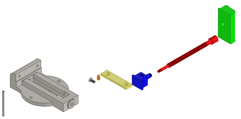
Figure 6.34: Placed Vice components within the new .iam file

4. Move your cursor over body.ipt in the Graphics window, and then right-click and select Grounded. This will ground the main component. With Constrain, it is important to do this for the first component.
5. Click and drag guide.ipt in the Graphics window near the body.ipt file you just grounded. This is the first component we will constrain with both Joints and Constraints.
6. Select the Assemble tab, select Joint, and then select Cylindrical from the dropdown. This will allow the component to rotate about the axis defined.
7. For the first reference, select the geometry of guide.ipt, as shown in Figure 6.35:

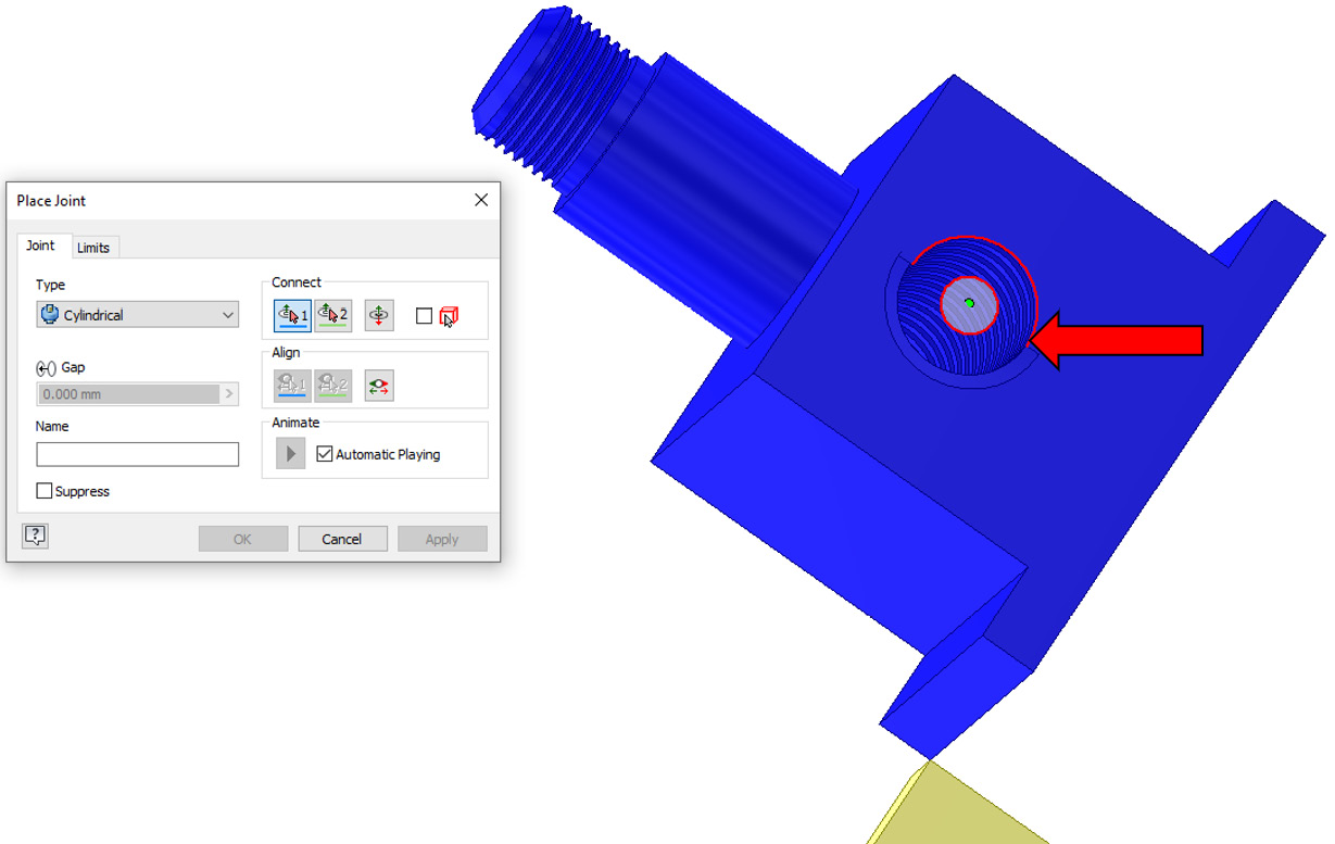
Figure 6.35: The first reference to select

For the second reference, select the geometry of the body, as shown in Figure 6.36:

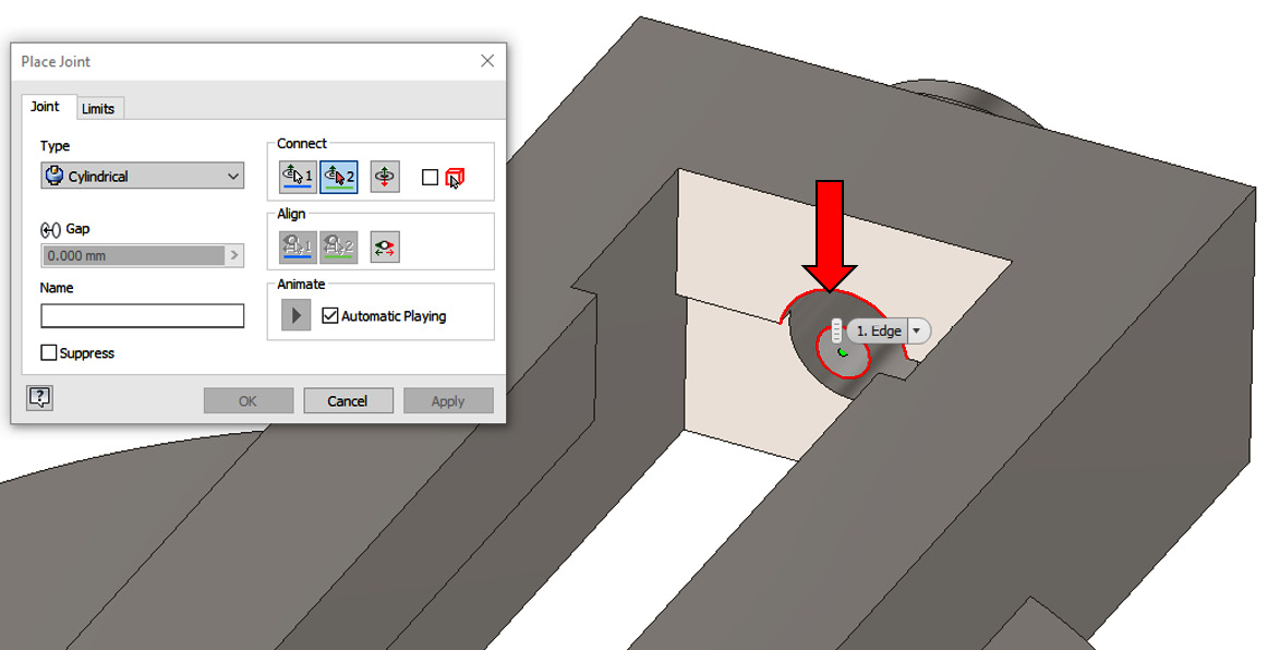
Figure 6.36: The second reference to select

Then, select OK.

8. The first joint has been applied, but as you can see, the component is still not properly defined, in relation to other components. You may find that guide.ipt can move inside body.ipt, as a Contact Set has not yet been defined; we will come onto Contact Sets in a few more steps. But for now, we will now define the component further.
9. Select Constrain from the Assemble tab.
10. Select Angle Constraint from the options and then select the face of guide.ipt, as shown in Figure 6.37:

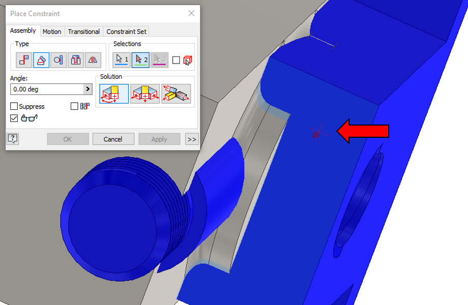
Figure 6.37: The first reference to select for the Angle Constraint

11. For the second reference, select the geometry of guide.ipt, as shown in Figure 6.38. Then, select Directed Angle from the options and leave the angle as 0 degrees by default. This will orientate the component and further define its allowable DOF. Select OK to complete.

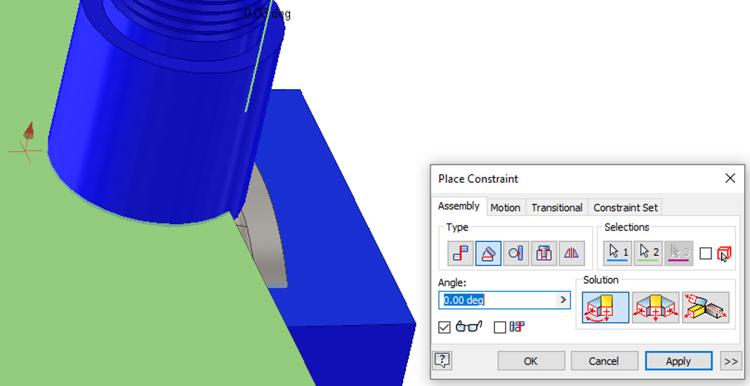
Figure 6.38: The second reference for the Angle Constraint with Directed Angle selected

12. No limits or Contact Sets have yet been applied to the allowable movement of these components. We can observe that none have been applied by clicking and dragging guide.ipt, and you should be able to slide it within body.ipt:

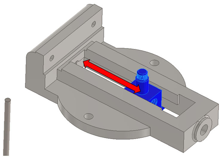
Figure 6.39: Allowable DOF

13. To further define these components, we can establish a Contact Set. This will stop the two components from going through each other when moved and start to establish some real-world physics in the model.

In the model browser on the left of the screen, select guide.ipt and body.ipt. Right-click and select Contact Set from the menu.

14. To turn the Contact Set on, navigate to the Inspect tab, and select Activate Contact Solver. If you click and drag the guide, it will only move bi-directionally within body.ipt and will not collide and merge with the body.ipt geometry. Select Activate Contact Solver to turn off the feature.
15. In the Graphics window, click and drag sliding jaw.ipt so that it is near body.ipt.
16. In the Assemble tab, select Joint, and then select Cylindrical as the option.
17. Select the first reference, as shown in Figure 6.40:

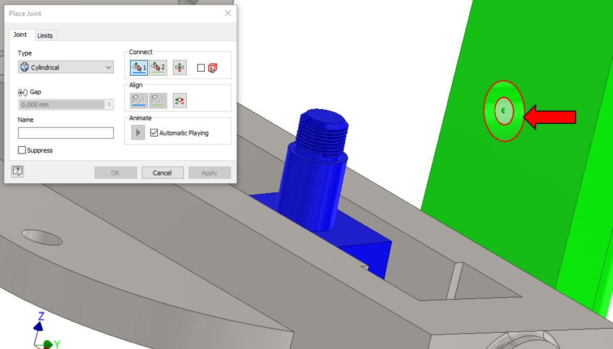
Figure 6.40: The first reference for sliding jaw.ipt

For the second reference, select the geometry shown in Figure 6.41:

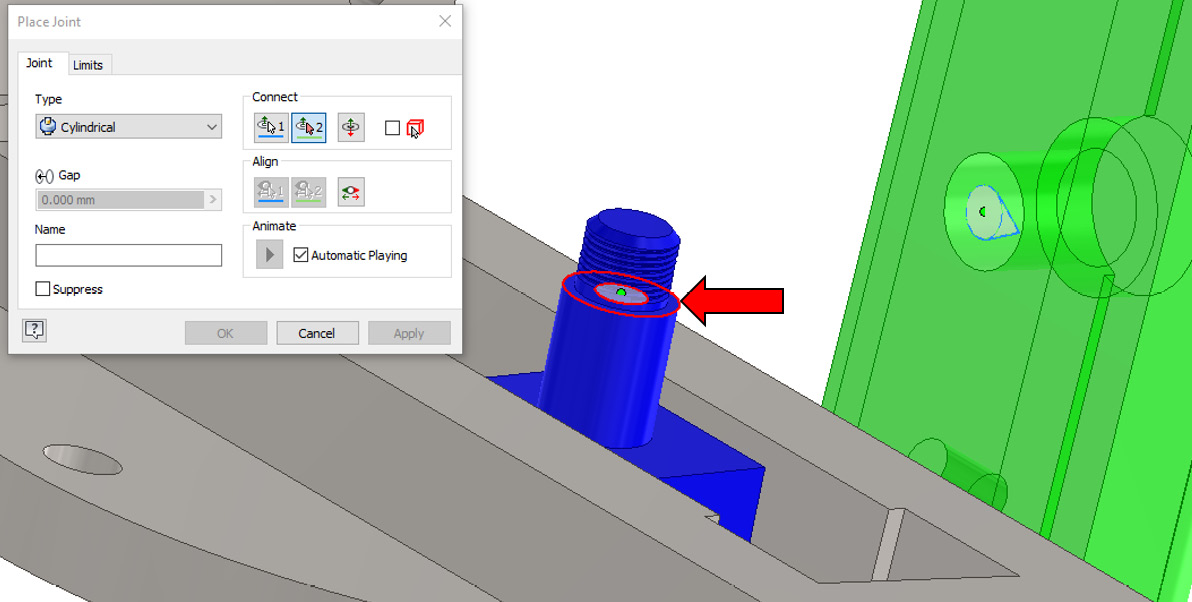
Figure 6.41: The second reference for sliding jaw.ipt

18. Ensure that sliding jaw.ipt is in the correct orientation, as per Figure 6.42. If not, select the flip icon highlighted in Figure 6.42 to flip the component to the correct orientation:

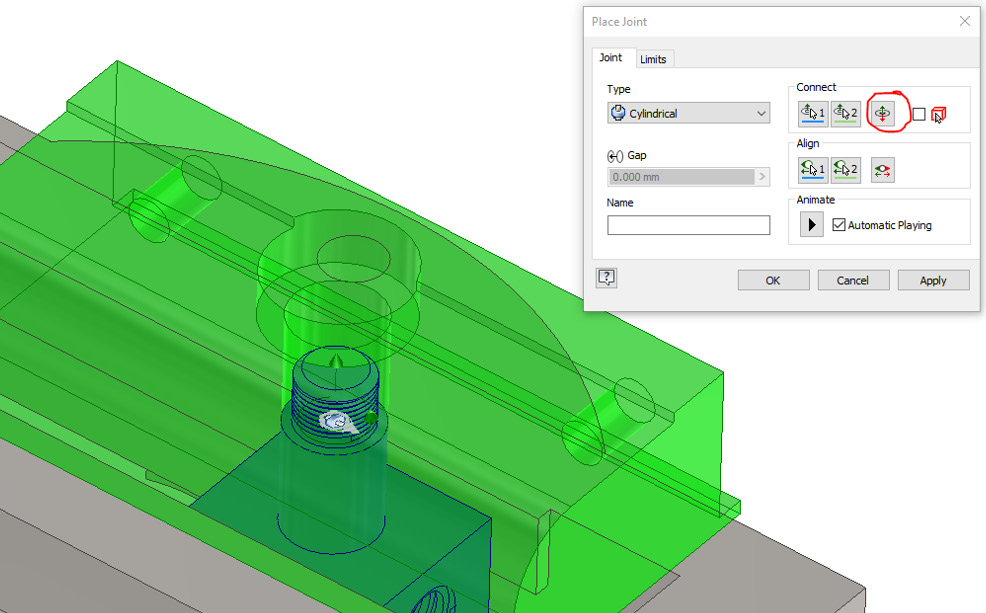
Figure 6.42: The flipping of the sliding jaw.ipt Cylindrial Joint if required

To complete the joint, select OK.

19. We now need to apply some Mate Constraints to further define sliding jaw.ipt. Select Constrain, and then Mate.
20. Select the bottom face of sliding jaw.ipt as the first reference, as shown in Figure 6.43:

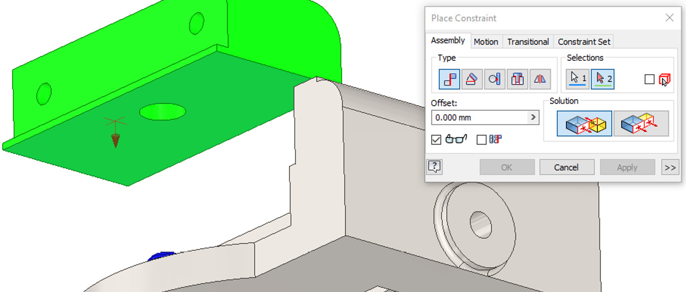
Figure 6.43: The first reference of the Mate constraint for sliding jaw.ipt

For the second reference, select the face of body.ipt, as shown in Figure 6.44. Then, select Apply:

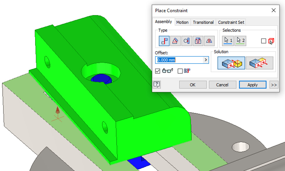
Figure 6.44: The second reference of the Mate constraint for sliding jaw.ipt

21. With the Place Constraint menu still active, select Angle as the Constraint type.

For the first reference, select the face of sliding jaw.ipt, as shown here:

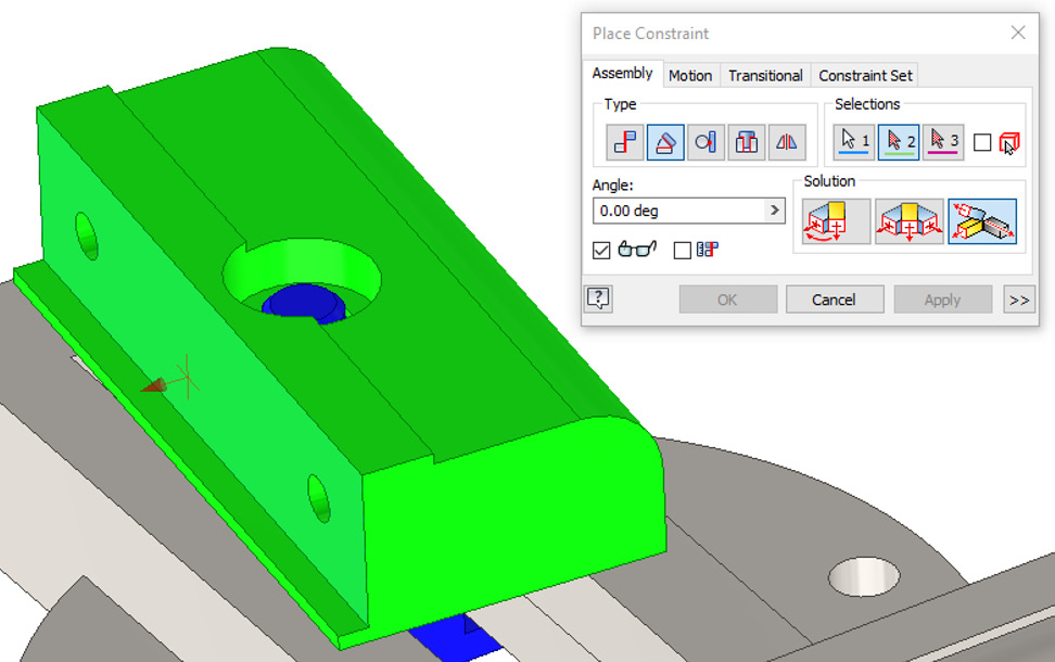
Figure 6.45: The first reference of the Angle constraint for sliding jaw.ipt

For the second reference, select the geometry shown in Figure 6.46:

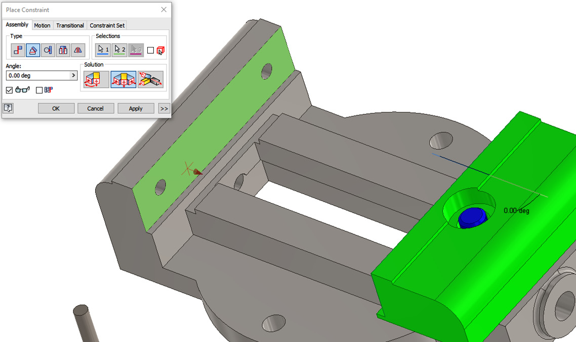
Figure 6.46: The second reference for the Angle Constraint for sliding jaw.ipt

Select Undirected Angle as the Solution option, and keep the value at 0 degrees as default. Select OK to complete.

This results in sliding jaw.ipt and guide.ipt moving as one within the constraints of body.ipt.

22. Click and drag the face plate in the Graphics window so that it is near body.ipt.
23. Select Joint, and then Cylindrical as the type, and then select the first reference as the geometry, as shown in Figure 6.47, on face plate.ipt:

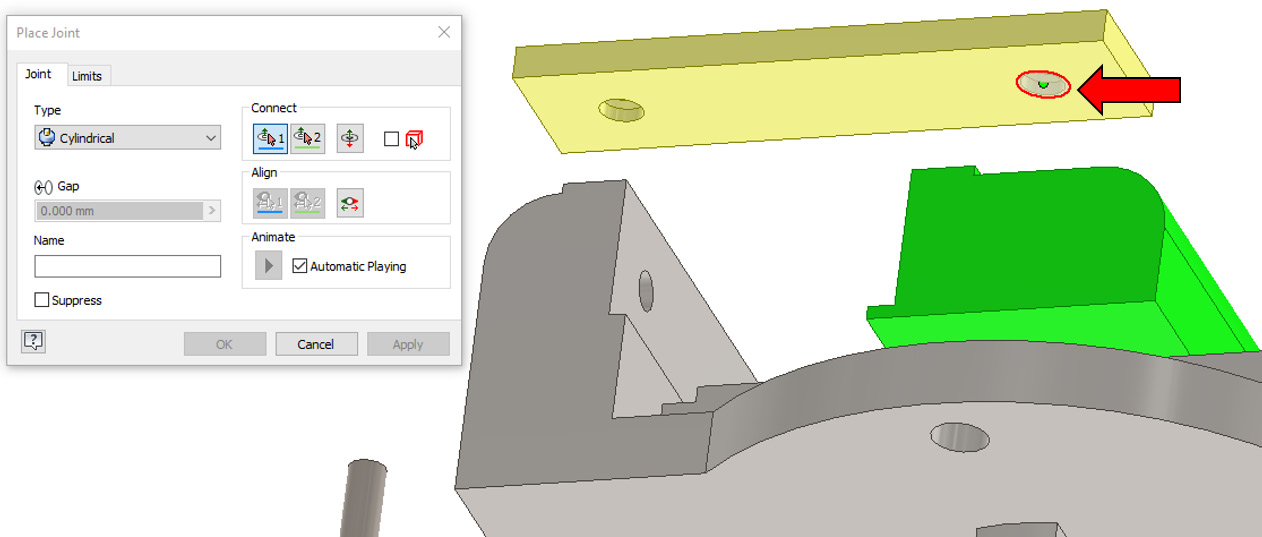
Figure 6.47: The first reference of the Cylindrical Joint for the face plate

For the second reference, select the corresponding hole feature of body.ipt, as shown in Figure 6.48:

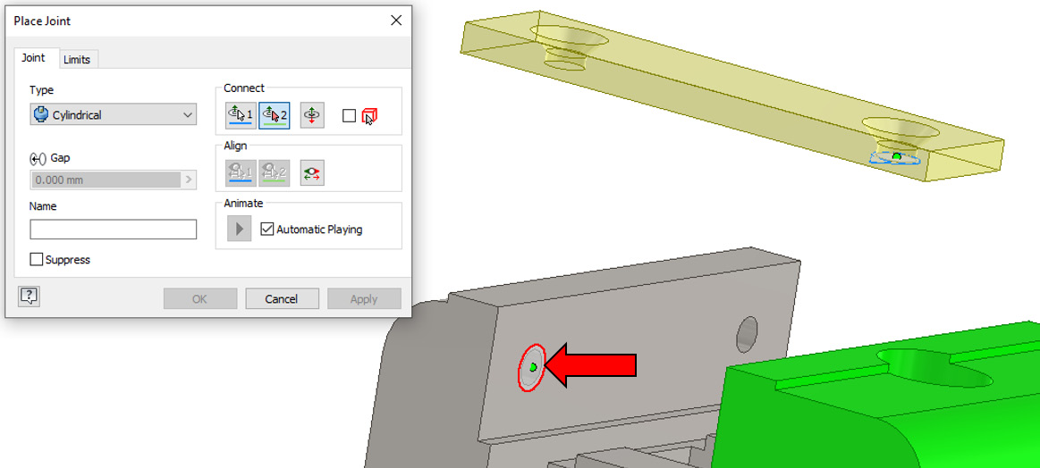
Figure 6.48: The second reference of the Cylindrical Joint for the face plate

If required, select Flip Component to ensure that the face plate is positioned in the correct orientation, as shown in Figure 6.49:

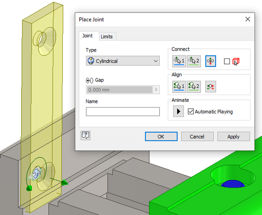
Figure 6.49: The face plate flipped during the Joint operation if required

Select OK to complete.

24. Create and apply a Mate Constraint between the center lines of the holes of both face plate.ipt and body.ipt, as shown in Figure 6.50. Select OK to apply:

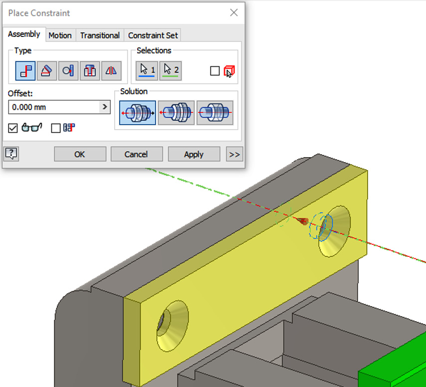
Figure 6.50: The Mate constraint applied to the centerlines of each hole in the face plate and body

25. The face plate still has DOF and can be pulled away. Click and drag the face plate away from the body in the Graphics window.
26. Select Constrain, then select Mate, and apply it to the geometry referenced in Figure 6.51:

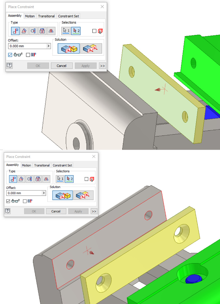
Figure 6.51: The two references selected to perform the Mate constraint

27. In the Graphics window, click and drag screw cap.ipt so that it is near face plate.ipt in the assembly.
28. Select Joint, and then select Rotational from the options. Proceed to select the edge of screw cap.ipt as the first reference, as shown in Figure 6.52:

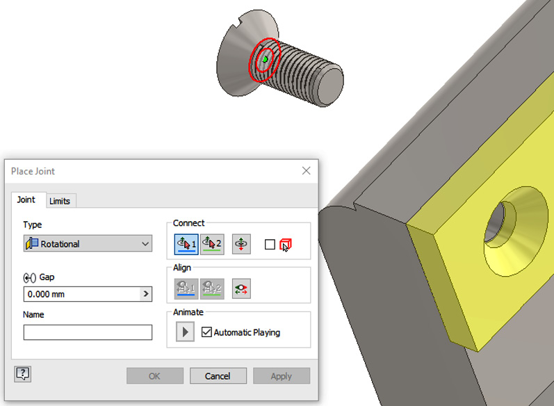
Figure 6.52: The first reference of the Rotational Joint for screw cap.iam

Then, select the following geometry as the second reference for this Joint, as shown in Figure 6.53:

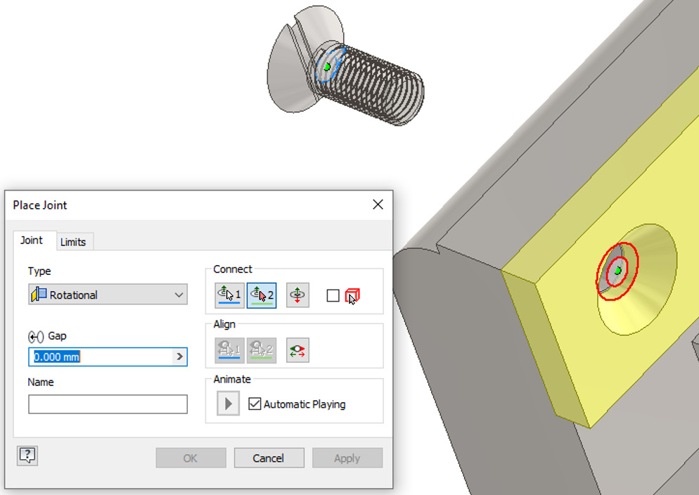
Figure 6.53: The second reference of the Rotational Joint for screw cap.iam

29. You may have to select Flip component to ensure that screw cap.ipt is in the correct orientation, as shown in Figure 6.54:

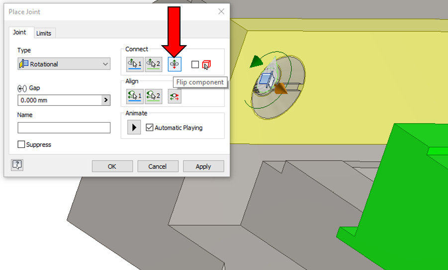
Figure 6.54: The flipped screw cap to move the component to the correct orientation

30. Select OK to complete.
31. As an optional extra step, you can also mirror screw cap.ipt about the center of the assembly to place another instance of it in the corresponding hole, as shown in Figure 6.55:

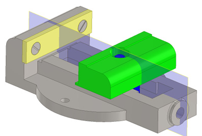
Figure 6.55: Optional step – mirroring screw cap.ipt across a midplane to create another instance on the corresponding hole

32. Click and drag the power screw.ipt toward body.ipt.
33. Select Joint, and then select Rotational as the Joint type.
34. For the first reference, select the geometry of power screw.ipt, as shown in Figure 6.56:

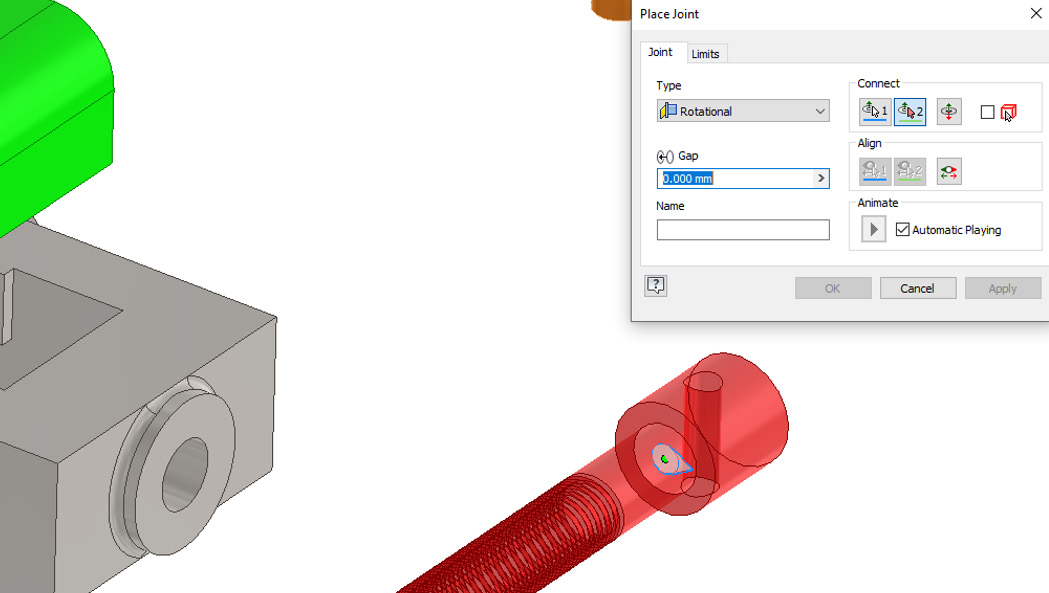
Figure 6.56: The first reference for the Rotational Joint of the power screw

For the second reference, select the geometry shown in Figure 6.57:

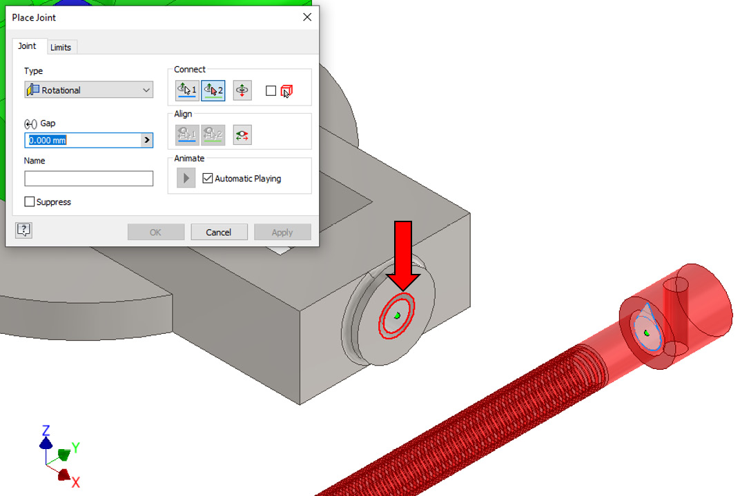
Figure 6.57: The second reference for the Rotational Joint of the power screw

Select OK to apply.

Pulling the sliding jaw in the assembly back and forth will not engage the power screw to turn, as a translational motion has not been defined. Therefore, the Joints and Constraints that we have applied are independent of one another. Translational Joints and motion can be applied in Inventor and will be covered in the Applying and driving Motion constraints recipe.

35. Select Constrain, and then select Mate. Place a Mate Constraint on the centerline of the cap and arm, as shown in Figure 6.58. Select OK to complete:

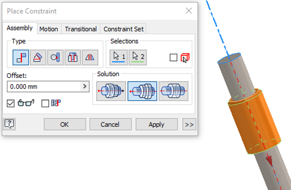
Figure 6.58: The Mate Constraint on the cap and arm

36. Create a second Mate Constraint from the top face of the arm and the inside face of the cap, as shown in Figure 6.59:

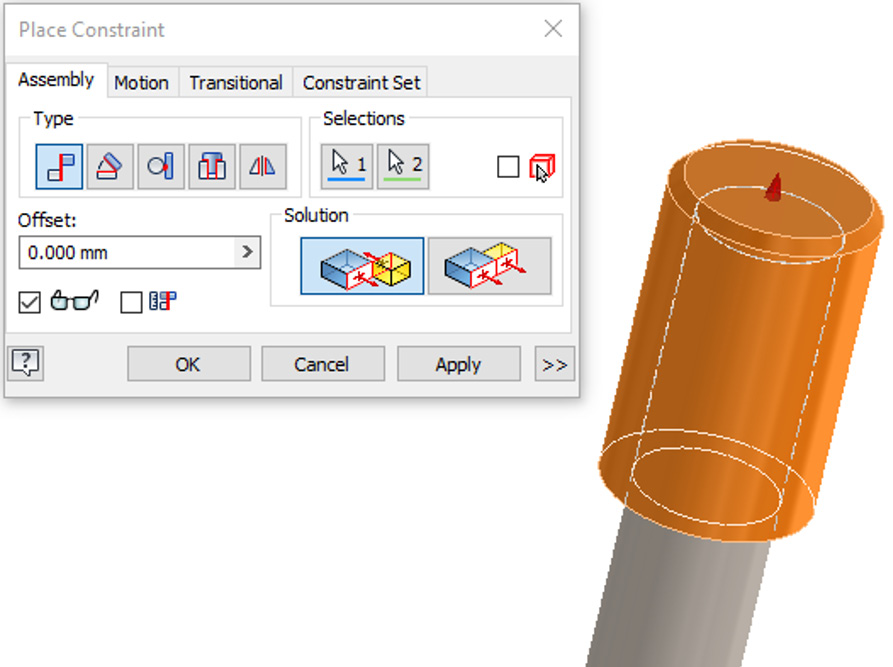
Figure 6.59: The Mate Constraint from the top face of the arm and the inside face of the cap

37. Create another Mate Constraint between the center of the arm and the center bore of the power screw, as shown in Figure 6.60:

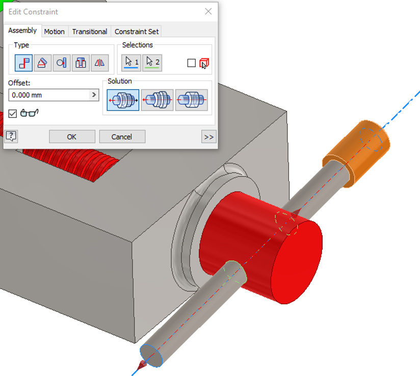
Figure 6.60: The Mate Constraint between the center of the arm and the center bore of the power screw

You have used a combination of Joints and Constraints to assemble several parts into an assembly, where DOF have been defined, ready for contact sets to be established.

Applying and driving Motion constraints

It is sometimes necessary to drive and examine motion between parts within an assembly to assess the end function and performance, and to detect possible collisions of components. With Motion constraints, you can apply and drive specified movement between parts.

In this recipe, you will apply Motion constraints to two spur gears, resulting in them being driven from a Motion constraint and meshing correctly.

Getting ready

To begin this recipe, you will need to access the Chapter 6 folder and open Gear Assembly.iam.

How to do it…

To begin, ensure that you have Gear Assembly.iam open. The two spur gears have already been created for you using the Spur Gear Design Accelerator, and they have also been locked into position with existing Constraints so that they can only rotate freely about the central axis.

To begin, we will examine the allowable movement and existing relationships in the assembly:

1. Expand the Relationships folder by selecting + next to the Relationships folder in the model browser. Here, you can see the existing Constraints that have already been applied to the gears to fix them into position at the correct distance.
2. Move your cursor over one of the gears in the Graphics window. Then, click, hold, and drag your cursor in a circular motion. You will see that the gear selected will rotate freely in position. The rotating of one gear does not affect another, and the teeth at this point will collide with each other:

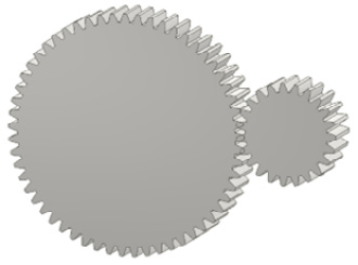
Figure 6.61: The gears rotate freely independent of one another and are not meshing correctly

We will apply Motion constraints to enable them to rotate with each other, and for the gears to mesh correctly.

3. In the Design tab, select the Spur Gear command from the ribbon.
4. In the Spur Gears Component Generator window, highlight the desired gear ratio default value. Right-click and select Copy, as shown in Figure 6.62.

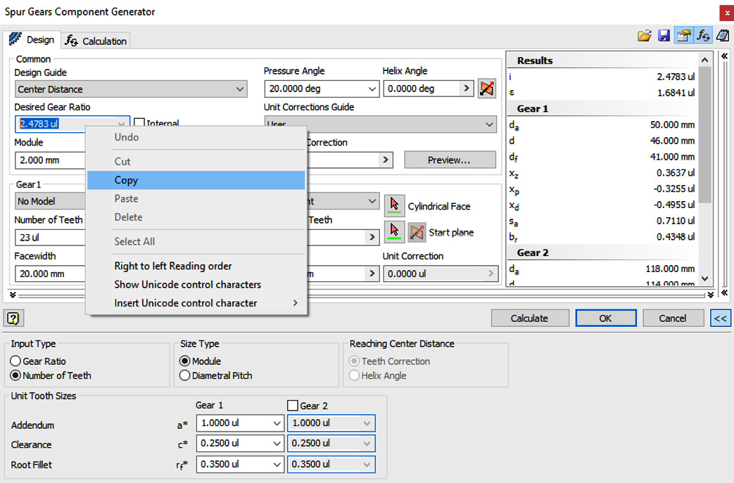
Figure 6.62: The Spur Gears Component Generator window, copying the gear ratio

Hit x to close the Spur Gears Component Generator window.

5. From the Assemble tab, select Constrain. Select the Motion tab within the Place Constraint window.
6. In Ratio, paste the ratio from the clipboard, which should be 2.4783 ul:

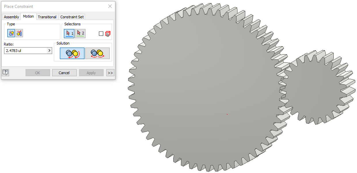
Figure 6.63: The Motion tab selected and a ratio of 2.4783 ul applied

7. Now, we need to select reference geometry for the Motion constraint. Navigate to the area shown in Figure 6.64, and select a flat face of the “bottom land” of the second gear:

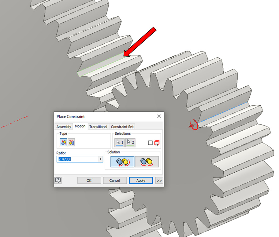
Figure 6.64: Selecting the first reference for the Motion constraint

8. Select a flat face of the “bottom land” of the second gear for the second reference:

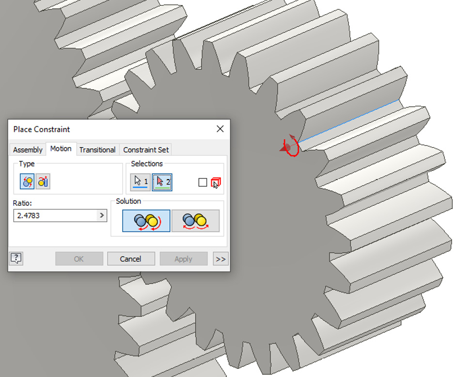
Figure 6.65: Selecting the second reference for the Motion constraint

Select OK to complete the Motion constraint.

9. In the Graphics window, move your cursor over one of the gears, and then click, hold, and drag your cursor in a circular motion. Both gears turn together because of the Motion constraint. However, they are still not meshing correctly:

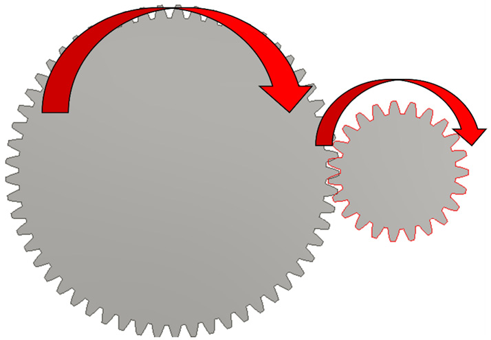
Figure 6.66: The gears rotate together but they do not mesh correctly

10. Navigate to the Relationships folder in the model browser, and expand + next to Relationships. Right-click on the Rotation 1 Motion constraint and select Suppress from the menu.
11. Select Front View on the ViewCube.
12. Click, hold, and drag one of the gears in the Graphics window so that they are aligned and meshed correctly:

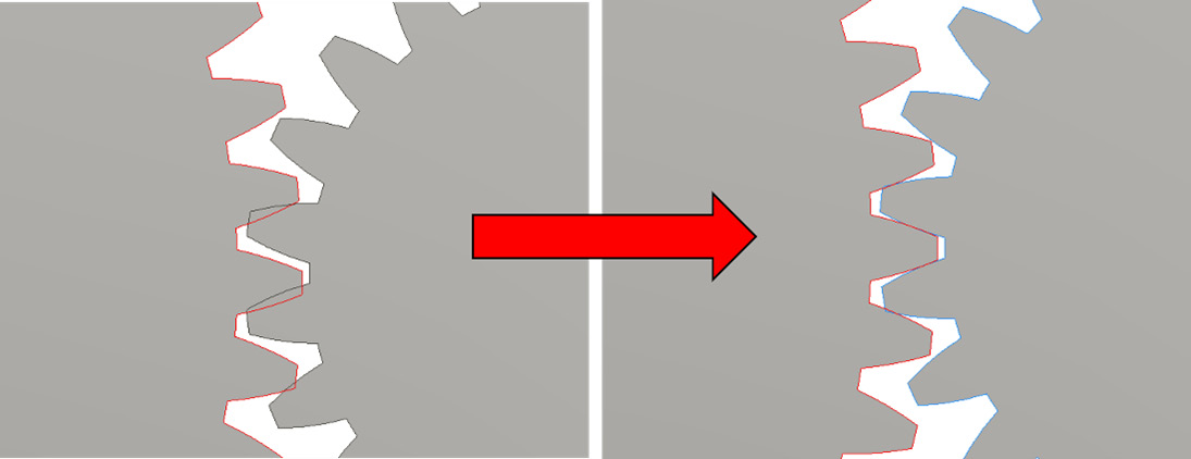
Figure 6.67: Gears meshing correctly

13. Right-click on Rotation 1 from the Relationships folder in the model browser and select Edit:
14. In the Edit Constraint window, select Reverse as the Solution option.
15. Navigate to the Relationships folder in the model browser, and expand + next to Relationships. Right-click on the Rotation 1 Motion constraint and select Suppress from the menu to unsuppress the Motion constraint.
16. In the Graphics window, move your cursor over one of the gears, and then click, hold, and drag your cursor in a circular motion. Both gears turn together because, and now the teeth mesh correctly.
17. Now, we will create an Angle constraint to drive the gear assembly automatically. Select Constrain from the Assemble tab.
18. Select Angle as the type, and for Solution, select Directed Angle.
19. For the reference, select YZ Plane of the first gear and XZ Plane of Gear Assembly.iam:

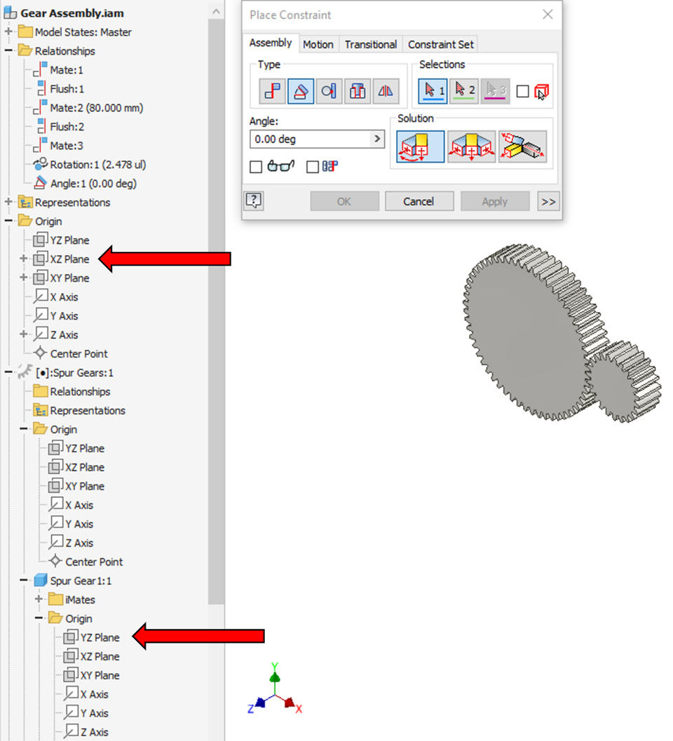
Figure 6.68: Planes to select for the Angle constraint

Select Apply to complete. Then, close the Place Constraint window.

20. In the model browser, right-click on Angle 1 Constraint and select Drive.
21. Change the End degree to 360 deg. Select the Forward button to drive the gears. Both gears will rotate and mesh correctly:

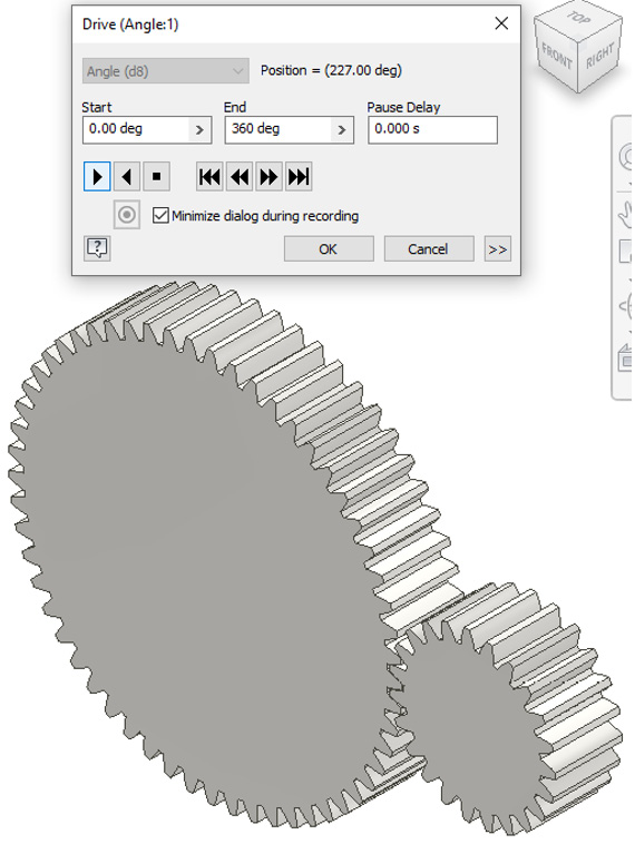
Figure 6.69: The End degree configured and Forward selected

You have applied Motion constraints to a set of gears and driven them with an Angle constraint to show the movement and correct meshing of the teeth.

Duplicating and replacing components in an assembly

Within an assembly, you can duplicate and replace components with ease. In many instances, you will need to duplicate or replicate parts or subassemblies – for example, standard components such as fasteners.

In this recipe, you will learn how to automatically place and size a fastener, and then replace and change the fastener. You will also learn to mirror and then pattern the component within an assembly. All these techniques should be combined when modeling assemblies in Inventor, as they maximize your efficiency and result in you having to recreate repeating geometry.

Getting ready

To begin this recipe, you will need to access and open Flange Assem.iam. This can be found in the following folder directory: Inventor 2023 Cookbook | Chapter 6 | Flange.

How to do it…

Ensure that you have Flange Assem.iam open in Inventor. In this recipe, we will begin the first steps of how to automatically place and size a fastener, replace and change the fastener, and then mirror and pattern the component within an assembly:

1. In the Assemble tab, under Place, select the dropdown and select Place from Content Center. This allows us to browse the Content Center library of standard parts within Inventor and specify the exact fastener we require.
2. Within the Place from Content Center window, we can browse for the content we require. In this case, we require a Hex Head bolt that is flanged. In Category View of the window, browse the following: ISO | Fasteners | Bolts | Hex Head- Flanged:

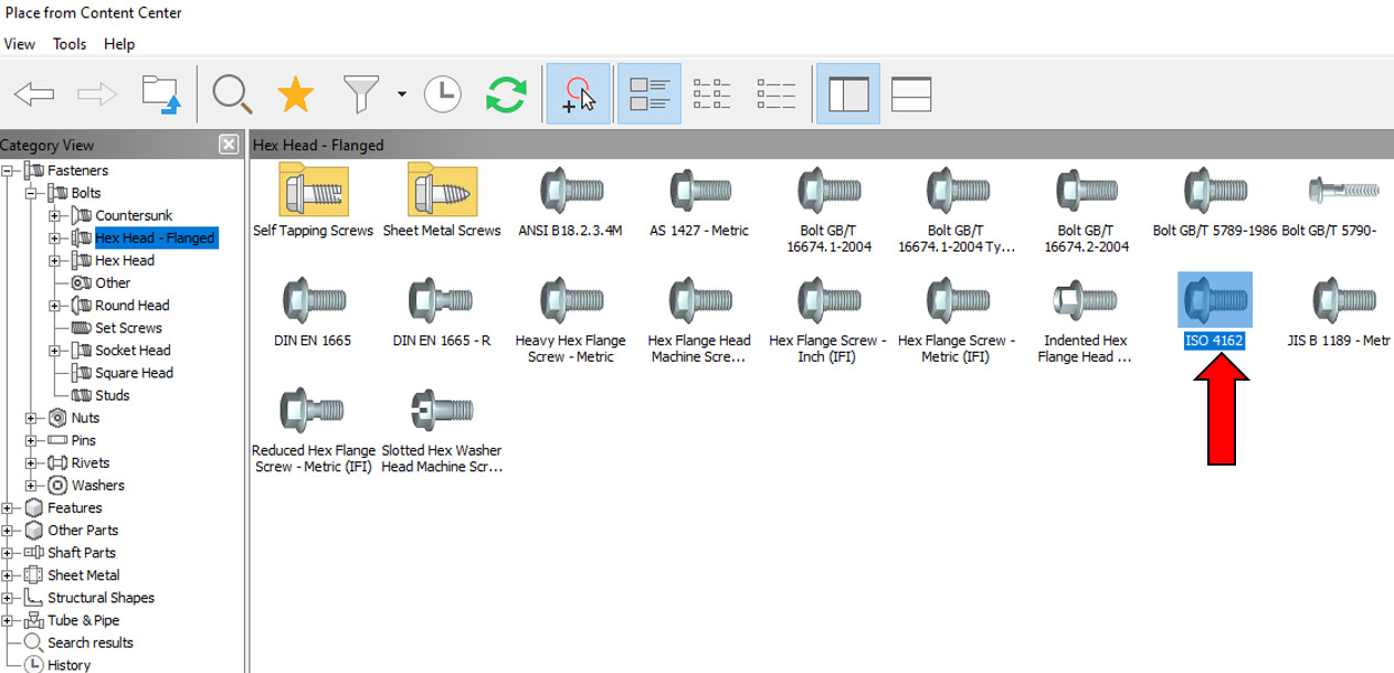
Figure 6.70: Selection of the ISO 4162 Bolt via the Content Center

Then, select the ISO 4162 Bolt, followed by OK. You can also use the filters to specify content based on a standard that you work in, such as ISO, ANSI, and more. A search functionality is also available, and using the star icon, you can mark content that you use frequently as a favorite.

3. Upon selecting OK in step 2, the ISO 4162 bolt will appear on your cursor within Inventor. The bolt can be placed with a left click; however, if that is done, additional constraints will have to be defined to place the bolt correctly. Instead, hover the bolt over one of the tapped holes in the flange.
4. As you hover the bolt over the tapped hole, Inventor will work to read the hole information, in the model, and resize the fastener to the correct size for that hole. Once complete, the fastener will preview, and a green tick may appear, signifying that Inventor has correctly resized your chosen fastener to the hole:

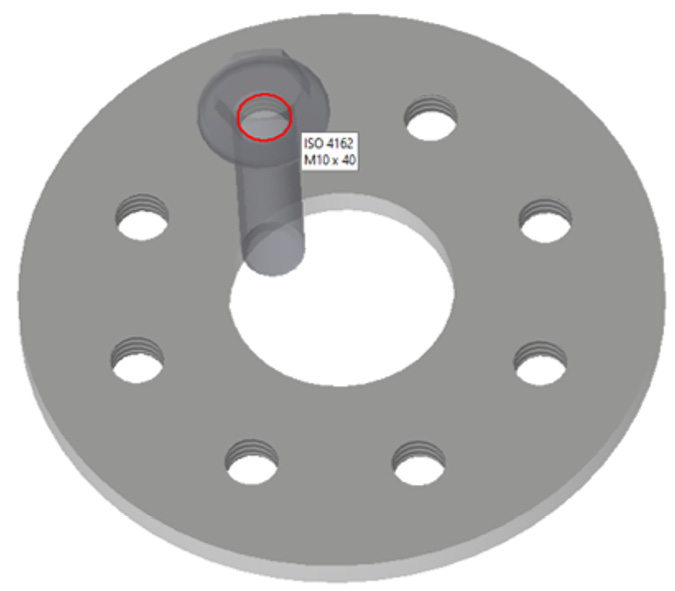
Figure 6.71: A preview of the fastener resized to the hole diameter

5. Once the fastener has updated, as shown in Figure 6.71, right-click and select Change size:

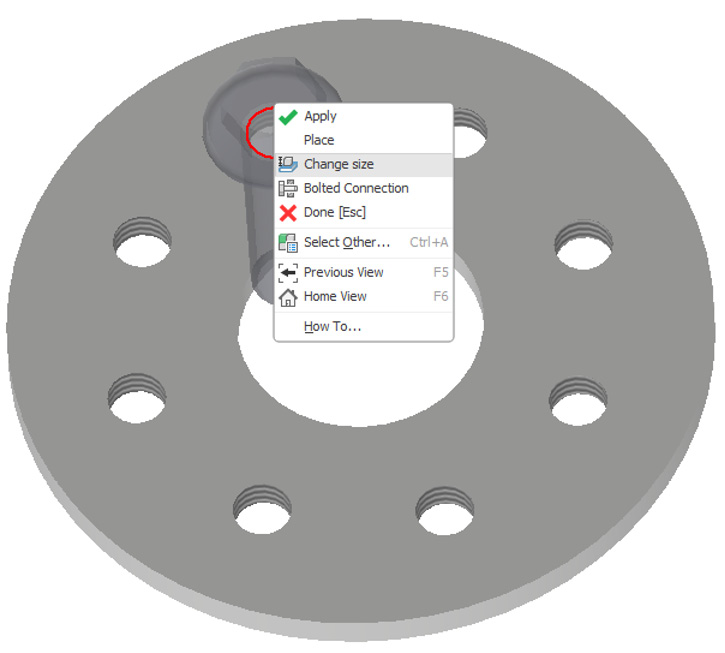
Figure 6.72: Resizing of the previewed fastener

Before placing the bolt in the flange, we need to adjust the length of the bolt.

6. In the next window, we can further define the fastener before placement. Change Nominal Length from 40mm to 45mm, and select OK. The defined ISO 4162 bolt is placed in the flange.
7. Upon placing a component, you may need to change it at a later stage. To do this, right-click on the fastener in the Graphics Window, and select Replace from Content Center.

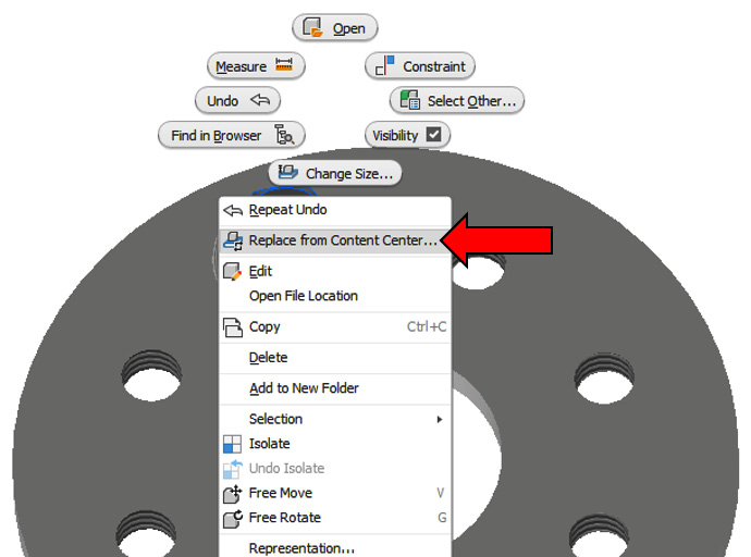
Figure 6.73: Replace from Content Center…

You can also replace components with parts you have created yourself by right-clicking on the component, selecting Component, and then either choosing Replace or Replace All to replace all in the series.

8. In Place in the Content Center window, select the JIS B 1189 – Metric bolt. Select OK.
9. Select M10 as Thread designation and leave Nominal Length at *22.
10. Select OK, followed by OK again. The previously placed ISO 4162 bolt has been replaced with the JIS B 1189 bolt. This has been automatically resized and constrained to the assembly, so no further constraint work is required to define this.
11. There are a number of holes remaining without bolts, and there are several duplication techniques we can apply to solve this. The first is a mirror of a component within an assembly. Expand the Origin folder in the model browser, and highlight the YZ, XZ, and XY planes. Right-click and select Visibility:

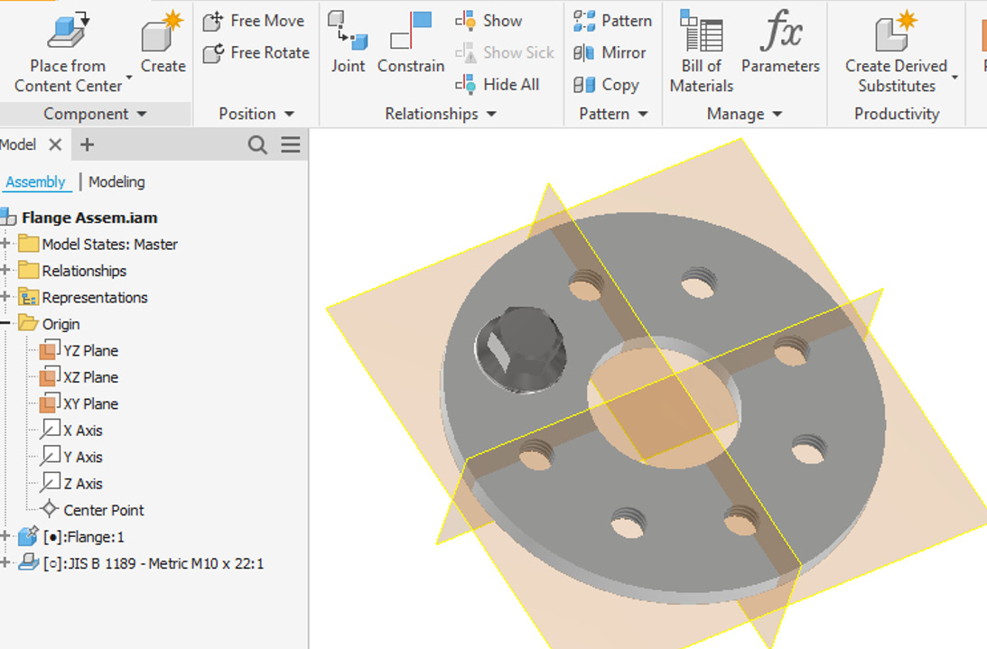
6.74: Origin planes made visible

12. In the Assembly tab, select Mirror.
13. Select JIS B 1189 as the component to mirror, and then select YZ Plane as the mirror plane:

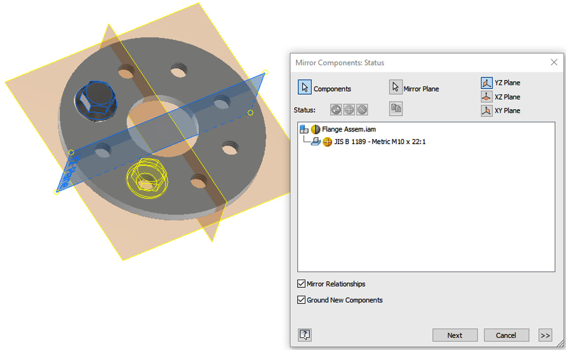
Figure 6.75: Mirror options to be selected

14. Select Next, followed by OK. The component has been mirrored into the correct position and is fully constrained:

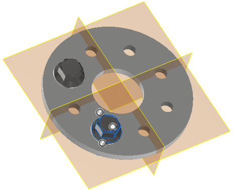
Figure 6.76: The mirrored component

Within the Mirror command, you can also mirror multiple components in one operation. Instead of Mirror, you can also use the Copy command, located under the Mirror command; this will allow you to freely place a copied part in the model, but further constraining will be required. You can also click and drag a component from the model browser into the Graphics window to create a copy.

15. There are still several fasteners required, and in this instance, repeated use of the Mirror command is not efficient. So, in the Model Browser, select JIS B 1189 – Metric M10 x 22.2, and press Delete.
16. We will now begin the more efficient process of using the Pattern commands to create and place the relevant fasteners. In the Assemble tab, select Pattern.
17. From the Pattern command, we can use several options to pattern and copy the selected component in the correct position. As holes inserted on the previous flange were created with a pattern, we can use this metadata in the part to assist with adding the bolt to the holes. Select JIS B 1189 – Metric M10 x 22.2 as the component to pattern.
18. For the feature pattern, select one of the remaining holes in the flange. The JIS B 1189 fastener will populate on these holes. Select OK to complete:

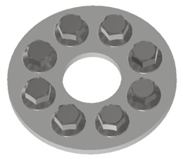
Figure 6.77: The completed assembly

You have automatically placed and sized a fastener from the Content Center, replaced and changed the fastener, mirrored it, and then used Feature Pattern to replicate the component within the assembly.

Creating and configuring a BOM

The BOM allows you to document and communicate the parts that make up an overall assembly for manufacture. The BOM is populated automatically, as parts are added to an assembly file, and Inventor will auto-populate this based on the metadata of the part files. In this sense, it is almost like a “live” document within the assembly file. Further customization and configuration can then be applied to the BOM to display specific information. You can also add parts to a BOM that do not have physical geometry, such as paint or grease, that may still be critical to the model, known as virtual components.

BOMs can also be exported as .txt or .csv files but will always remain within the assembly file itself and update as parts change in the assembly file.

In this recipe, you will learn how to do the following:

• Generate a BOM that lists components within the assembly
• Customize and edit properties in the BOM
• Create a virtual component in the BOM

Getting ready

To begin this recipe, you will need access to the Chapter 6 folder, and open Shaft Gear Motor.iam. This can be found in this folder directory: Inventor 2023 Cookbook | Chapter 6 | Shaft Gear Motor.

How to do it…

Ensure that you have Shaft Gear Motor.iam open in Inventor. In this recipe, we will create and configure a BOM:

1. With Shaft Gear Motor.iam open in Inventor, in the Assemble tab, select Bill of Materials.
2. This generates the BOM for that assembly. If subassemblies are included in the model, they will also be included. In this case, the assembly is made up of single parts only. Within the Bill of Materials menu, we can make all the modifications we require to the BOM. We will start by converting the BOM to a Parts Only list. This is important to do if you are working with embedded subassemblies, as without this, you will not be able to see them in the BOM. Select the Parts Only (Disabled) tab.
3. Then right-click on Parts Only (Disabled) and select Enable BOM View. A parts-only structure is now visible:

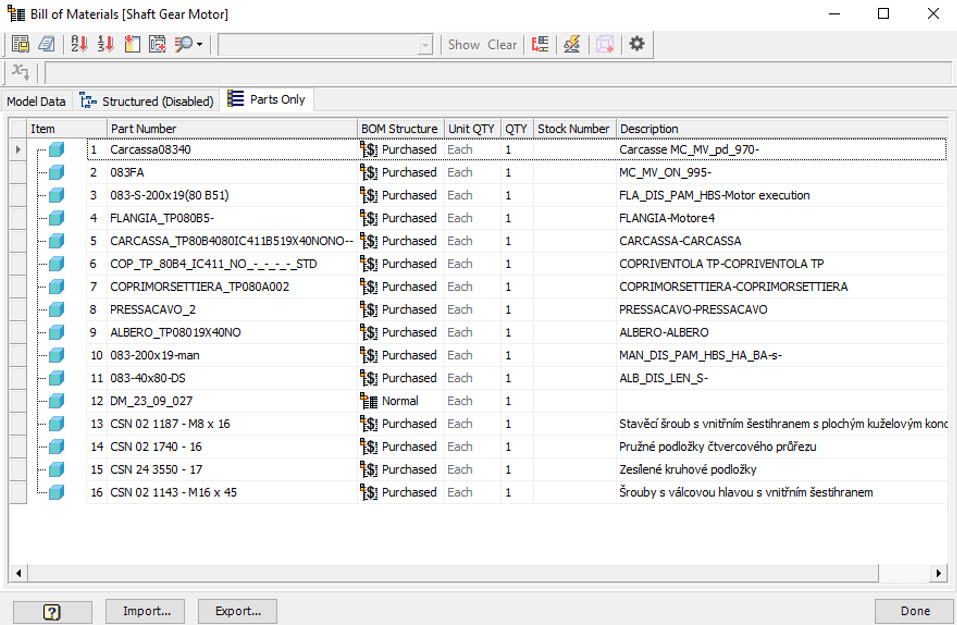
Figure 6.78: Parts Only enabled in the BOM

4. Columns and the information shown can be further customized, by dragging columns. Click and drag QTY and move it between Part Number and BOM Structure. The BOM will update:

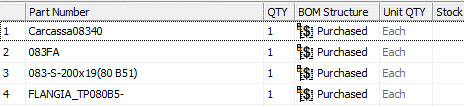
Figure 6.79: Columns updated in the BOM

5. Columns can also be taken out and added. Click and drag the Stock Number column until a black x icon appears, and then release the mouse. This will remove the column.
6. We will now insert additional columns of information into the BOM. Select the Choose Columns button in the Bill of Materials window:

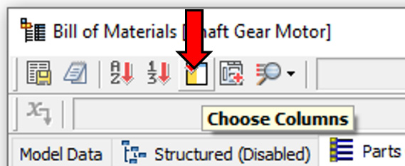
Figure 6.80: The Choose Columns button

7. In the Customization window that appears, double-clicking on a category will import this into the BOM, and all information will be automatically added. Browse the list and double-click Mass and then Material to add them to the BOM view. The columns will automatically update, based on the metadata of the parts:

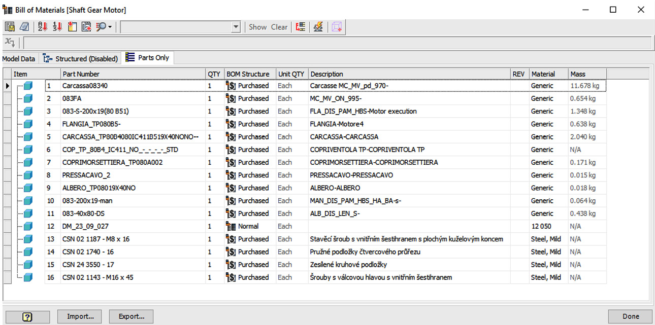
Figure 6.81: The updated BOM list with Material and Mass added

8. To show the live link between the BOM and the assembly file, we will update a material of any part and observe the Mass change within the BOM. Select Done on the BOM to close the menu.
9. In the model browser, right-click on the PRESSACAVO_2:1 part and select Edit.
10. In the Material selection tab, browse for and select PC/ABS Plastic:

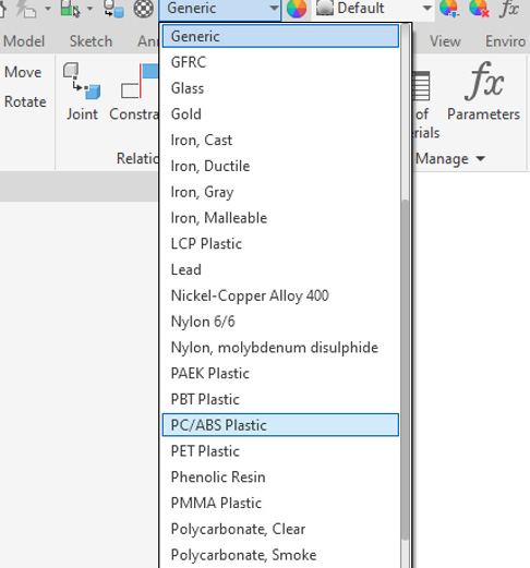
Figure 6.82: The PC/ABS Plastic material selected

11. Select Return in the ribbon to return to the assembly.
12. Select Bill of Materials, look down the list, and find the PRESSACAVO_2:1. You will see that the Material type and Mass have been updated to reflect the change made in the model:

Figure 6.83: Updated Material and Mass for PRESSACAVO_2:1

13. Quantities of parts can also be changed from within the BOM. It may be that in this part, you will supply some spare versions that may not necessarily be included in the CAD model. Double-click on QTY 1 next to PRESSACAVO_2:1 and type 4 to change the quantity in the BOM.
14. An important aspect of the BOM we can change is the BOM structure. This is used to provide a more accurate BOM, where further categorization of components can be defined. The five options available are as follows:
    • Normal: Default status for all components placed in an assembly file.
    • Phantom: Used to simplify a design. They exist in the model but are not included in the BOM and are excluded from quantity calculations.
    • Reference: Used in the construction of the assembly but not used in the design. This could, for example, be a skeleton model for a frame-like structure. Reference components are excluded from all BOM calculations.
    • Purchased: Used to denote parts that are purchased and not manufactured.
    • Inseparable: These are components that must be damaged to take them apart – for example, welded parts or tight interference fitting parts.

You are free to change parts’ BOM structure in the BOM window. For the 083FA part, double-click on the Purchased BOM structure in the table. Then, select Normal from the dropdown, which changes the BOM structure of the part:

Figure 6.84: The BOM structure changed from Purchased to Normal

15. The BOM can also be sorted and renumbered. To renumber a BOM, select the Renumber Items button:

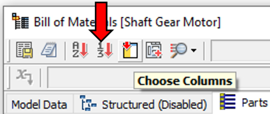
Figure 6.85: The Renumber Items button in the Bill of Materials window

16. In this example, we will change the start number to 2 and the increment to 2. Select OK to complete:

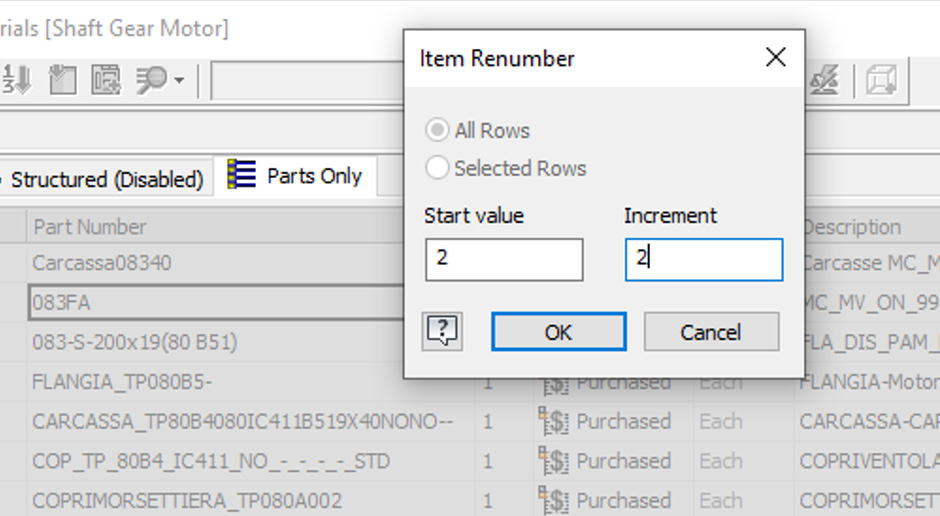
Figure 6.86: Item renumbering in the Bill of Materials window

The BOM will renumber as specified.

17. The BOM can also be sorted and reorganized with the Sort Items command. Select the Sort Items command:

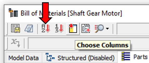
Figure 6.87: The Choose Columns command

18. Change the sorting fields, as shown in Figure 6.88, using the drop-down menu, and select OK. This will sort the BOM as per the sorting specifications:

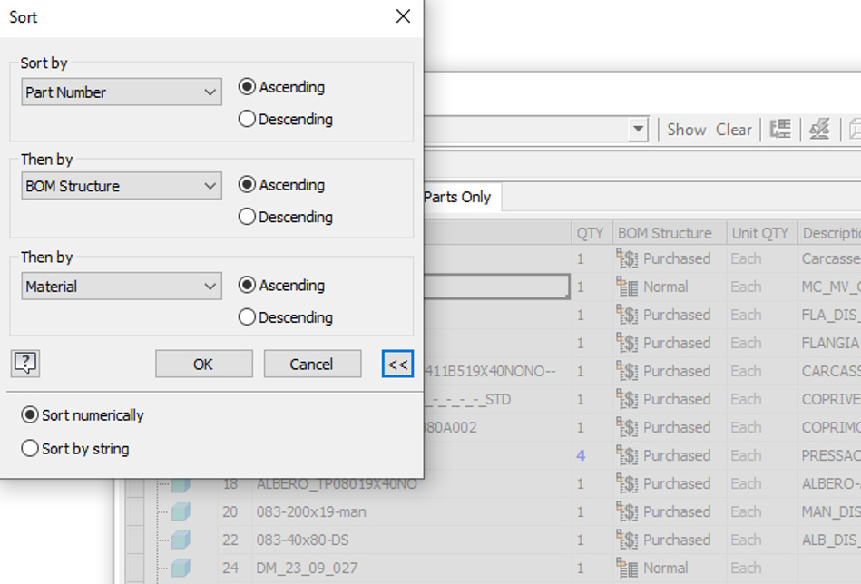
Figure 6.88: Sorting columns in the BOM

19. Close the Bill of Materials window, as we will now create a virtual component called Grease. This is a component that’s important to the design, which we need in the CAD but is impossible to model.
20. In the Assembly tab, within the component panel, select Create.
21. Create a new component called Grease, select Virtual Component, and select Purchased under Default BOM Structure. Select OK to complete:

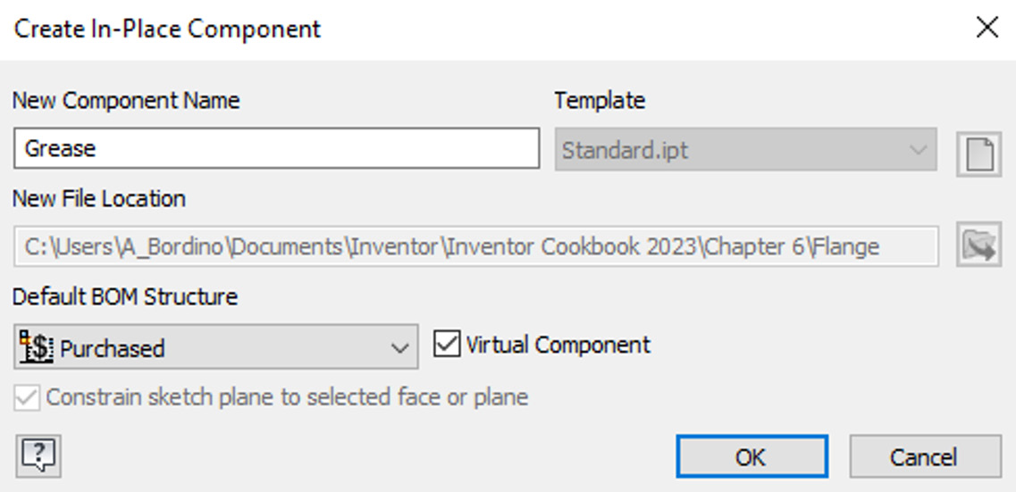
Figure 6.89: Defining the name and default BOM structure of the virtual component

22. We now need to create a parameter to define the base quantity of Grease, measured in millimeters. Right-click on the Grease component in the model browser. Select Component Settings.
23. Select the Edit Parameters button:

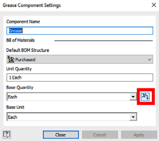
Figure 6.90: The Edit Parameters button in Grease Component Settings

24. Select Add Numeric in the Parameters dialog box.
25. Create a new parameter called Base_Quantity, set the units to ml, and the equation to 1 ml. Select Done to complete:

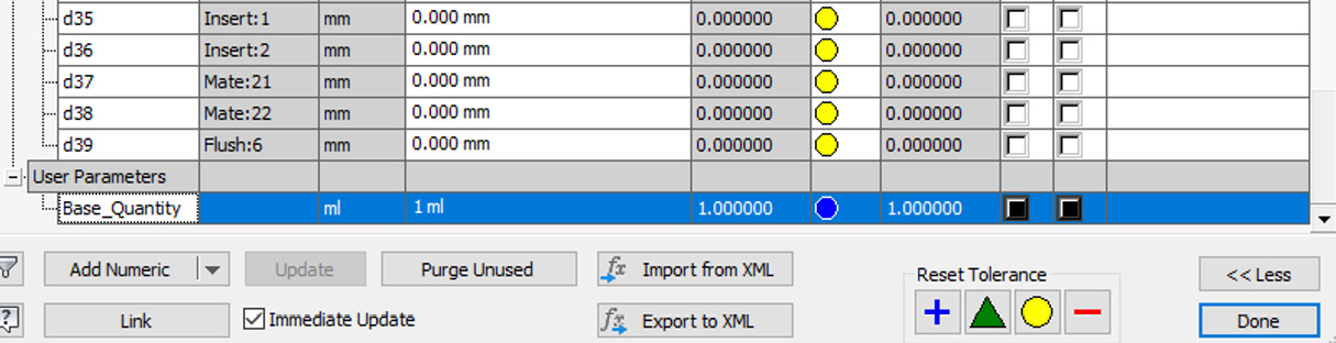
Figure 6.91: A new parameter created for the virtual Grease component

26. We will now change the base quantity to the correct unit. Change Base Quantity to Base_Quantity (1ml), and select OK:

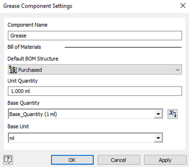
Figure 6.92: Adding Base_Quantity (1 ml) to the virtual component

27. We will now change Grease so it has the correct quantity. So, select Bill of Materials, then in the Grease item, change the quantity from 1ml to 100.000 ml:

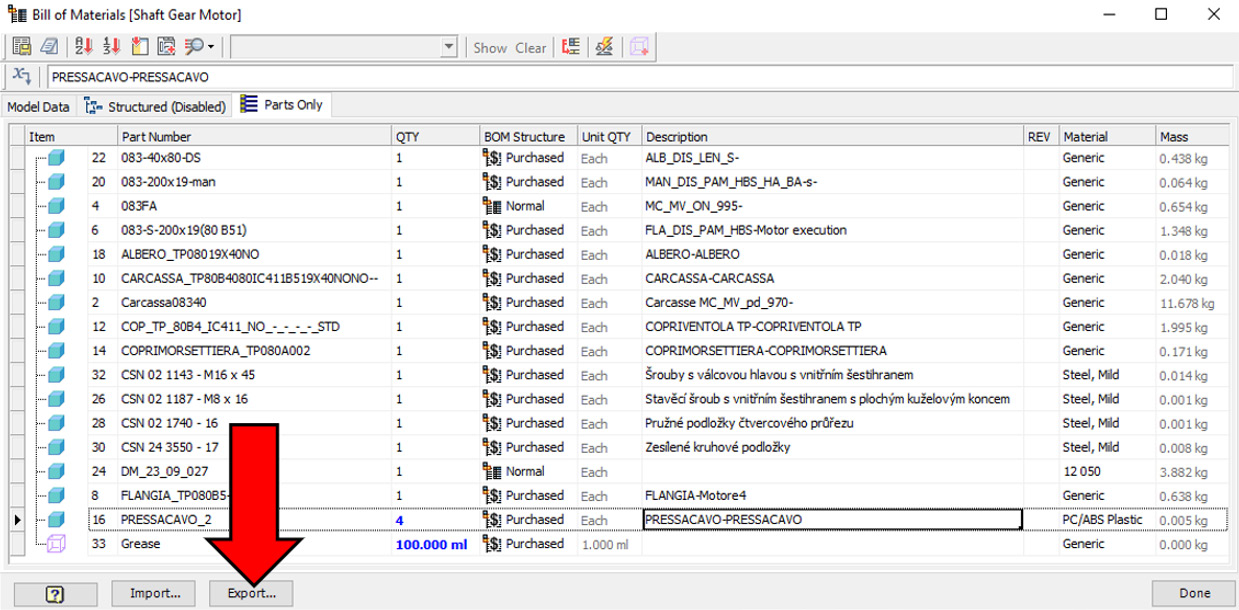
Figure 6.93: The quantity of the virtual grease component changed from 1 ml to 100.000 ml

28. A BOM can also be exported as a .csv or text file. To do this, select Export….
29. In the Windows menu, browse and save your BOM as an .xml file, named TEST BOM.

You have generated and customized a BOM for components within an assembly, edited properties, added a virtual component, and exported the BOM in an .xml file.

Detailing and customizing a BOM in a drawing file

In this recipe, you will create a General Arrangement (GA), a drawing of an existing assembly, add and customize a BOM to the drawing sheet, and auto-balloon all components within the drawing.

Getting ready

To begin this recipe, you will need access to the Chapter 6 folder and Shaft Gear Motor.iam. This can be found in this folder directory: Inventor 2023 Cookbook | Chapter 6 | Shaft Gear Motor.

How to do it…

Ensure that you have Shaft Gear Motor.iam open in Inventor. To create a GA drawing, and add and customize a BOM to the drawing sheet, we will follow these steps:

1. Select File, New, Metric, ISO.idw, and then select Create.
2. In the new ISO.idw file, select Base View, and browse Shaft Gear Motor.iam. Use the ViewCube to rotate the base view so that the ViewCube is displaying the top view, as shown in Figure 6.94. Change Scale to 1:4:

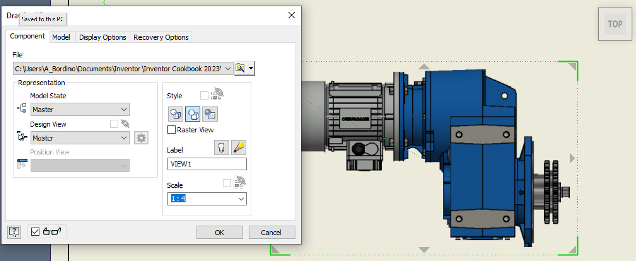
Figure 6.94: The top view of the shaft gear motor

3. Move the cursor toward the top right of the drawing screen and left-click to place a projected ISO view of the assembly. Right-click and select OK to complete:

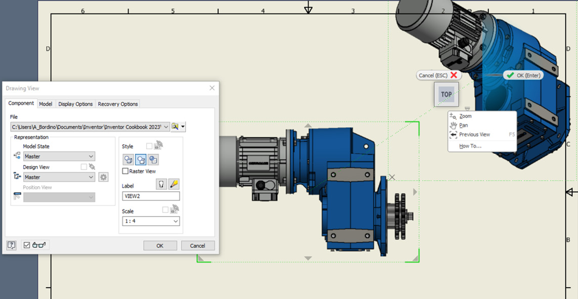
Figure 6.95: The ISO view added

4. Click and drag the two placed views so they resemble Figure 6.96:

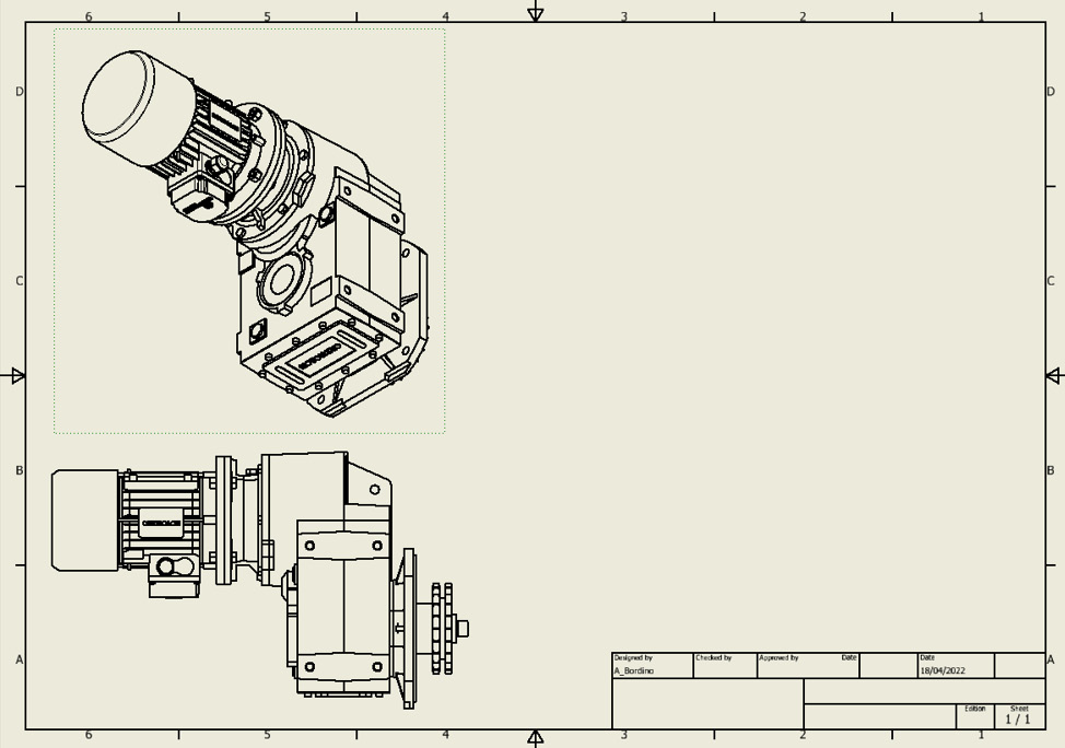
Figure 6.96: Drag the placed views in this position on the drawing sheet

5. Select the base view and hit Delete. Select OK to complete. Drag the ISO view to the bottom left of the drawing sheet.
6. Double-click the ISO view. Using the ViewCube, move the view to the position shown in Figure 6.97 to re-orientate it. Then, select Shaded for Style. Select OK to complete:

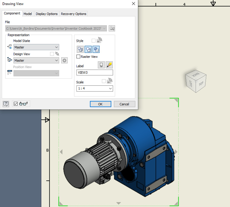
Figure 6.97: The completed ISO view

7. Select the Annotate tab. Navigate to the Table commands and select Parts List.
8. Select ISO View on the drawing sheet as the referenced view.
9. Select Parts Only from the BOM View options:

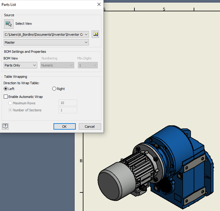
Figure 6.98: The Parts List options to select

10. Select OK. A preview BOM will appear on the cursor. Left-click at the top right of the drawing sheet to place this. The BOM will be placed here.
11. Double-click on the newly placed BOM in the drawing.
12. As in the Creating and configuring a BOM recipe, you can customize a BOM in the drawing environment the same way you did in the assembly file. Select 1 in the QTY column for the 083FA part and change it to 5:

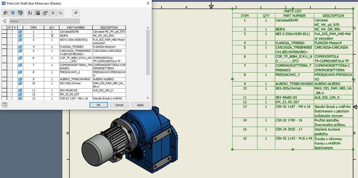
Figure 6.99: Customizing the BOM in the drawing environment

13. Select the Column Chooser command at the top left of the Parts List dialog box.
14. Browse for Mass and Material, and select them. Then, select Add to move them into the BOM. Select OK to complete, followed by OK again. The parts list or BOM is updated on the drawing sheet:

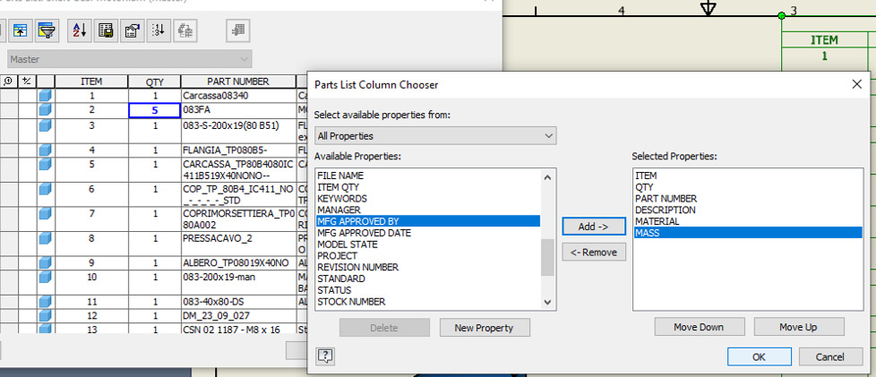
Figure 6.100: Choosing additional columns for the BOM

15. To annotate and auto-balloon, in the Annotate tab, select Auto Balloon.
16. Select the ISO view on the drawing sheet.
17. You can now select the specific items to balloon from the assembly. In this case, draw a box around the whole view to select all parts. Inventor will ignore duplicate parts in the auto balloon by default:

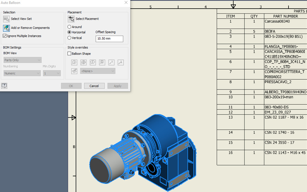
Figure 6.101: All parts selected from the assembly for the auto balloon

18. Select the Select Placement button.
19. Select Around from the list. Move your cursor toward the drawing view on the drawing sheet. You will see that previews of the balloons populate. When ready, left-click and select OK to place:

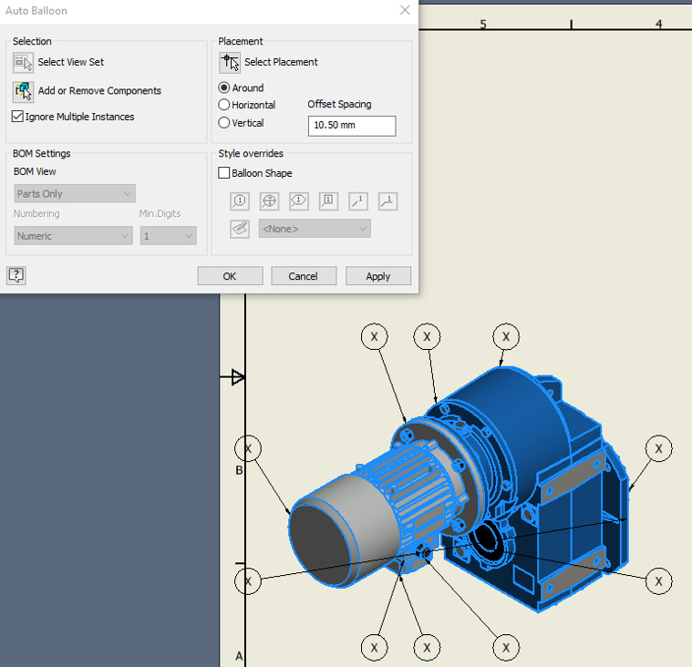
Figure 6.102: A preview placement of the auto balloon

If balloons are placed in an undesirable location, they can be moved freely after placement with a click and drag.

20. The auto balloon has now correctly numbered the parts of the assembly on the drawing. If changes are made to the file, the BOM and the balloons will update if required:

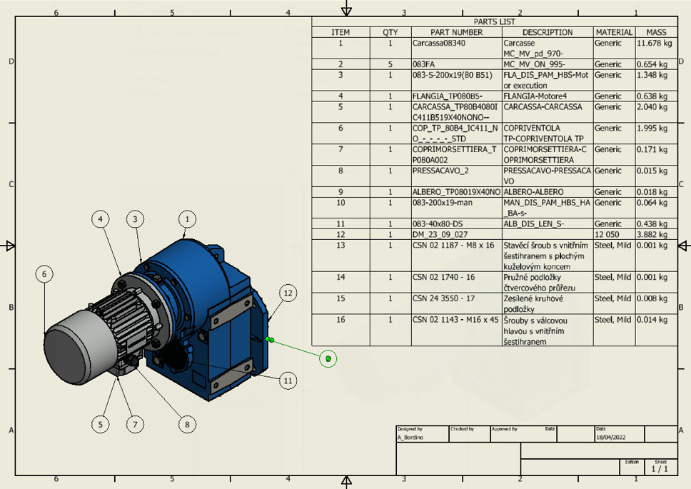
Figure 6.103: The completed Auto Balloon operation

You have created a new drawing of an existing assembly, placed an isometric view, added a BOM and customized it, and then used Auto Balloon to detail the components.

Model credits

The model credits for this chapter are as follows:

• Brake (by Gabriel Medeiros): https://grabcad.com/library/brake-51/details?folder_id=10984917
• Vice (by Ahmed Habashy): https://grabcad.com/library/vice-86/details?folder_id=4922098
• SHAFT GEAR MOTOR WITH ACCESSORIES (by Dařena Miroslav) https://grabcad.com/library/shaft-gear-motor-with-accessories-1