Chapter 9: Comet for Natural Language Processing

Natural Language Processing (NLP) is a subfield of artificial intelligence, aimed at making computers capable of understanding human natural language in the form of both text and spoken words. You can use NLP applications to build virtual assistants, such as Alexa or Siri, sentiment analyzers, document translators, chatbots, and document classifiers. In this chapter, you will review the main concepts behind NLP, including the basic NLP pipeline and how to transform texts into data structures.

Over the last year, different open source tools and libraries have been implemented to perform NLP, including Spark NLP, spaCy, and Natural Language Toolkit (NLTK). In this chapter, you will review the Spark NLP library and see how to integrate it with Comet. We will focus on how to perform NLP on texts, although you can also apply NLP to audio documents.

Training a good NLP model can be very time- and process-consuming because it usually requires a huge quantity of texts as input. For this reason, you can find many pretrained models available on the web, such as those provided by Hugging Face, a very popular website, used by about 5,000 organizations, including Google, Facebook, Microsoft, and Amazon Web Services. In this chapter, you will review the most popular hubs for pretrained models.

In the last part of this chapter, you will implement a practical use case that uses the Spark NLP library and track the results in Comet.

This chapter is organized as follows:

• Introducing basic NLP concepts
• Exploring the Spark NLP package
• Setting up an environment for Spark NLP
• Using NLP, from project setup to report building

Before starting to review the basic NLP concepts, let’s install the required software needed to run the examples described in this chapter.

Technical requirements

We will run all the experiments and codes in this chapter using Python 3.8. You can download it from the official website, https://www.python.org/downloads/, choosing the 3.8 version.

The examples described in this chapter use the following Python packages:

• comet-ml 3.23.0
• pandas 1.3.4
• scikit-learn 1.0

We already described these packages and how to install them in Chapter 1, An Overview of Comet, so please refer back to that for further details on installation.

In addition, the running examples will need other specific requirements, which will be described in the Setting up the environment for Spark NLP section of this chapter.

Now that you have installed all the software needed in this chapter, let’s look at how to use Comet for NLP, starting by reviewing some basic concepts.

Introducing basic NLP concepts

NLP is a subfield of artificial intelligence, aimed at analyzing and synthesizing human language and speech. You can use these models for different purposes, such as translation, chatbots, spam filters, grammar correction software, and voice assistants. NLP has become very popular in the last few years, thanks to the spread of huge quantities of text that can be analyzed to build very domain-specific tools.

The section is organized as follows:

• Exploring the NLP workflow
• Classifying NLP systems
• Exploring NLP challenges
• Reviewing the most popular models’ hubs

Let’s start from the first step, exploring the NLP workflow.

Exploring the NLP workflow

The following figure shows the simplest NLP workflow:

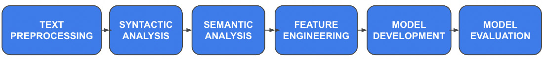
Figure 9.1 – The simplest NLP workflow

The workflow involves the following steps:

• Text preprocessing – This step involves preparing text for further analysis. Typically, during this phase, the text is split into sentences, and stop words are removed. Then, sentences are split into tokens and, finally, normalized.
• Syntactic analysis – This step involves sentence parsing and Part of Speech (PoS) tagging.
• Semantic analysis – This step involves Named Entity Recognition (NER) and concept recognition.
• Feature engineering – In this step, you extract features to build a machine learning model or a rule-based system, which performs a specific NLP task, such as text classification or translation.
• Model development – This step involves the development of the model, which can be either a machine learning or a rule-based model. Usually, you can use a machine learning model for a classification task, while you can use a rule-based model to extract some patterns from text.
• Model evaluation – This final step calculates the performance of the developed model.

The following table shows an example of workflow, which includes sentence splitting, stop word removal, tokenization, PoS tagging, and NER, for the following text:

Yesterday I went to Rome. I visited the Colosseum.

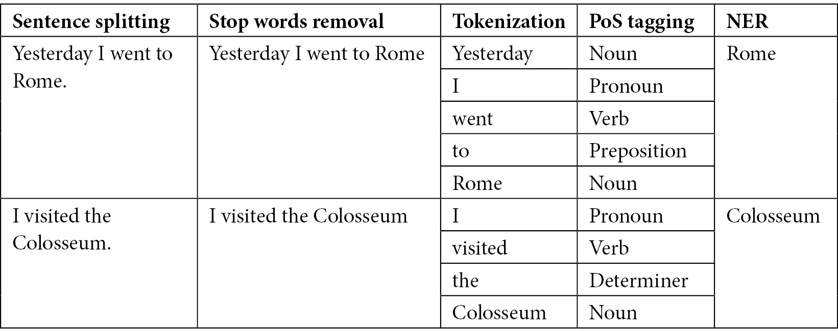
Figure 9.2 – A part of the NLP workflow for the text “Yesterday I went to Rome. I visited the Colosseum."

The text contains two sentences, separated by the intermediate dot (full stop). The stop word removal task simply removes the final full stop from each sentence. Tokenization splits each sentence into tokens, while PoS tagging recognizes the parts of speech for each token. Finally, NER recognizes two entities: Rome and Colosseum.

Now that we have reviewed the basic NLP workflow, we can move to the next step, classifying NLP systems.

Classifying NLP systems

Generally speaking, you can classify NLP systems into two big families:

• Functionality libraries – A functionality library is a collection of functions aiming at implementing some specific NLP tasks. Usually, these functions are independent of each other, and if, for example, you perform a PoS tagging task, the relative function also performs the operations that must be performed upstream, such as sentence splitting and tokenization. These libraries are good for research purposes, but they perform less well than the annotation libraries, since they do not provide any combination among the different tasks.
• Annotation libraries – An annotation library ensures that each NLP task is synchronized with the previous and subsequent ones, thanks to the concept of the document-annotation model. Thus, if you have to perform a PoS tagging task, you will first have to perform separately all the tasks that prepare the text for PoS tagging.

In this chapter, we will focus on Spark NLP, which is an annotation library.

Now that we have reviewed the basic classification of NLP systems, we can move to the next step, exploring NLP challenges.

Exploring NLP challenges

Although NLP has evolved enormously in recent years, thanks to the dissemination of large quantities of texts to analyze, many challenges still appear, including the following:

• Contextual words – A word may have multiple meanings, which depend on the context where it is inserted. Although a human can recognize the specific meaning easily, this process is not so trivial for a machine.
• Synonyms – Different words may have the same meaning. This issue is complementary to the previous one, but it has the same effects on machines, which may encounter difficulties associating the same meaning with different words.
• Irony and sarcasm – Usually, a word will be either positive or negative. However, when you use irony and sarcasm, you invert the original polarity of a word; thus, a negative word is used to express a positive concept, and vice versa. For a machine, recognizing irony and sarcasm can be very problematic because it associates a single polarity with each word.
• Ambiguity – This aspect refers to the possibility that a sentence has multiple interpretations. There are different levels of ambiguity, including lexical, semantic, and syntactic ambiguity.
• Errors in text or speech – It can happen that a word is not written correctly because it includes a typo or is misspelled. For a machine, recognizing this kind of error can be difficult.
• Colloquialisms and slang – Recognizing colloquialisms and slang in spoken language can be problematic for a machine, especially when the documents to analyze come in the form of audio.
• Domain-specific language – Some pretrained models work very well on generic texts, but they need to be adapted to specific domains. In this case, it may be difficult to find texts to train the models.

Now that we have reviewed some popular challenges of NLP, we can move toward the next step, an overview of the most popular model hubs for NLP.

Reviewing the most popular models’ hubs

Training an NLP model on large amounts of data can be time-consuming as well as resource-consuming. For this reason, over time, communities, companies, and researchers have combined their efforts and produced pretrained models that are ready to use. You can use these models directly as they are, or you can adapt them to a specific domain. There are several websites, or model hubs, that collect pretrained models that can be downloaded and used for free.

The most popular aforementioned model hubs include the following:

• Model Zoo
• TensorFlow Hub
• Hugging Face

Let’s briefly describe each hub, starting from the first one, Model Zoo.

Model Zoo

Model Zoo is a model hub for deep learning models, available at the following link: https://modelzoo.co/. Models are organized by category and framework. Categories include computer vision, NLP, generative models, reinforcement learning, unsupervised learning, and audio and speech.

Frameworks include TensorFlow, Caffe, Caffe2, PyTorch, and Keras. For each model, there is a detailed description that shows how to install and use it.

TensorFlow Hub

TensorFlow Hub contains pretrained models using TensorFlow, related to different categories, which include NLP for texts and audio, as well as computer vision tasks. For each model, you can find the description and a snippet of code on how to use it.

TensorFlow hub is available at the following link: https://tfhub.dev/.

Hugging Face

Hugging Face is a Python library, which also provides a model and dataset hub, available at the following link: https://huggingface.co/models. You can find pretrained models for NLP, image classification, reinforcement learning, and much more.

To use a specific pretrained model, you need to install the Hugging Face library and load the model from the library.

Comet is fully integrated with Hugging Face. For more details on how to use Comet with Hugging Face, you can read the Comet official documentation, available at the following link: https://www.comet.ml/docs/v2/guides/getting-started/tutorials/nlp-data/.

Now that we have reviewed some popular model hubs of NLP, we can move on to the next step, a review of the Spark NLP package.

Exploring the Spark NLP package

Spark NLP is an open source library for NLP released by John Snow Labs. It supports different programming languages, including Python, Java, and Scala. Spark NLP is widely used in production, since it is natively integrated with Apache Spark, a multi-language engine for large-scale analytics.

Spark NLP provides more than 50 features, including tokenization, NER, and sentiment analysis.

In this section, you will investigate the following aspects:

• Introducing the Spark NLP package
• Integrating Spark NLP with Comet

Let’s start from the first point, introducing the Spark NLP package.

Introducing the Spark NLP package

Spark NLP is an open source library built on top of Apache Spark and Spark ML (a machine learning library implemented on top of Apache Spark). The Spark NLP library provides almost all the NLP tasks, including tokenization, stemming, lemmatization, PoS tagging, sentiment analysis, spellchecking, and NER. The full list of implemented tasks is available in the Spark NLP official documentation, available at the following link: https://nlp.johnsnowlabs.com/docs/en/quickstart.

Spark NLP defines the following main concepts:

• Annotator
• Pipeline

Let’s investigate each concept separately, starting from the first one, the annotator.

Annotator

An annotator is either a Spark ML estimator or transformer. In Spark NLP, an estimator is an algorithm that you can train on a given DataFrame to produce a model, called a transformer. A transformer is a trained algorithm that can transform one input DataFrame into an output DataFrame. The difference between input and output DataFrames is that the input DataFrame contains features, while the output DataFrame contains predictions. The following figure shows how estimators and transformers are related to each other:

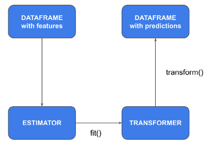
Figure 9.3 – The relationship between estimators and transformers in Spark ML

Spark NLP provides two types of annotators:

• An annotator approach, which extends the Spark ML estimator to implement the fit() method
• An annotator model, which extends the Spark ML transformer to implement the transform() method

Spark NLP also provides many pretrained annotator models, which have been already trained by someone else and are ready to use. You can check the NLP Models Hub website for the complete list of all the pretrained models, available at the following link: https://nlp.johnsnowlabs.com/models. All the pretrained models also provide the pretrained() method, which permits you to select the specific model to load, as shown in the following piece of code:

lemmatizer = LemmatizerModel.pretrained('lemma_antbnc', 'en')

The previous code loads the pretrained lemma_antbnc model.

All the annotators, whether an annotator approach or an annotator model, implement the following two methods:

• setInputCols(column_names): The list of input column names required by this annotator
• setOutputCol(column_name): The name of the output column containing the result of the current annotator

Now that we have reviewed the basic concepts behind annotators, we can move on to the next concept defined by Spark NLP, a pipeline.

Pipeline

A pipeline is an ordered sequence of stages, and each stage is either a transformer or an estimator. Each stage updates the DataFrame by adding new annotations, as shown in the following figure:

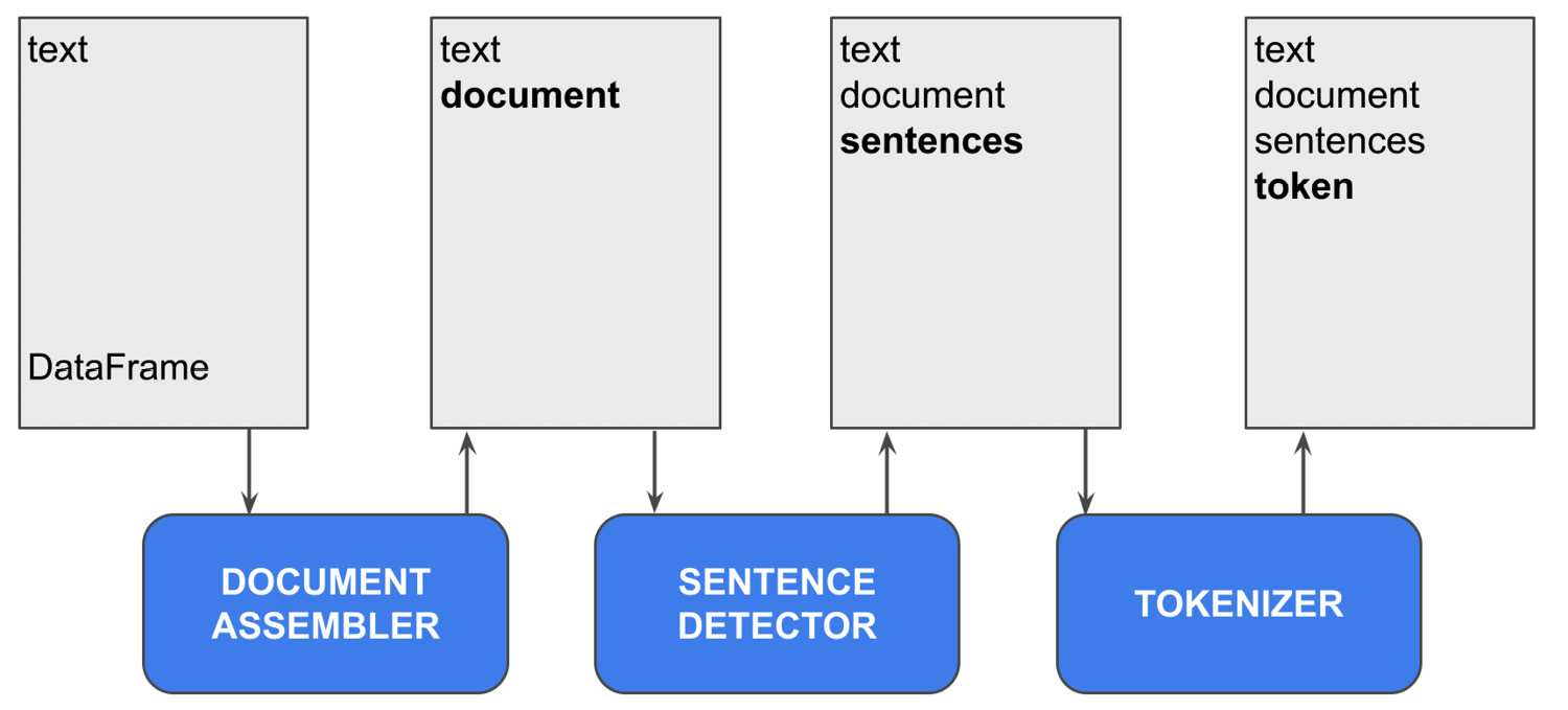
Figure 9.4 – A simple NLP pipeline

The previous figure implements a simple pipeline, composed of the following three stages:

• Document assembler – This Annotator is the initial stage of each Spark NLP pipeline. It creates the first annotation on the DataFrame, which is read by the next stage in the pipeline. The output column of this annotator is called a document.
• Sentence Detector – This annotator splits the document into sentences and adds a new annotation, called sentences, to the DataFrame.
• Tokenizer – This annotator tokenizes each sentence, and adds a new annotation, called token, to the DataFrame.

Similar to pretrained models, Spark NLP also provides pretrained pipelines, such as BasicPipeline, which implements sentence splitting, tokenization, lemmatization, stemming, and PoS tagging.

For more information on pipelines, you can read the Spark NLP official documentation, available at the following link: https://nlp.johnsnowlabs.com/docs/en/concepts.

Now that we have reviewed the basic concepts behind Spark NLP, we are ready to learn how to integrate Spark NLP with Comet.

Integrating Spark NLP with Comet

You can monitor your NLP experiments directly in Comet, either during the training process or at the end of an experiment. To integrate Spark NLP with Comet, you should create a CometLogger object, as follows:

from sparknlp.logging.comet import CometLogger 

logger = CometLogger()

The CometLogger class provides the following main methods:

• log_pipeline_parameters(): Logging the parameters of each stage of the pipeline in Comet
• log_visualization(): Uploading the NER visualization provided by Spark NLP Display to Comet
• log_metrics(): Logging evaluation metrics in Comet
• log_parameters(): Logging multiple parameters in Comet
• log_completed_run(): Submitting the results of training metrics once the pipeline training process is complete
• log_asset(): Uploading an asset to Comet
• monitor(): Monitoring the training of the model and submitting logs to Comet while the pipeline training process is running

For the complete list of methods, you can read the documentation, available at the following link: https://nlp.johnsnowlabs.com/api/python/modules/sparknlp/logging/comet.html.

You can access the experiment class defined in Comet through the logger.experiment field.

You can only use the monitor() and log_completed_run() methods for some annotator approach objects, such as a MultiClassifierDLApproach object. When you configure the pipeline to work with one of the supported annotators, you should enable logs, as well as set the path where to save them, as shown in the following piece of code:

from sparknlp.annotator import MultiClassifierDLApproach() 

PATH=/path/to/my/directory 

model = MultiClassifierDLApproach() 

      # add other configuration parameters 

.setEnableOutputLogs(True) 

      .setOutputLogsPath(PATH) 

We have used the setEnableOutputLogs(True) method to enable logs, and the setOutputLogsPath() method to set the path where to save logs. CometLogger will read the output of the log during the training process, as shown in the following piece of code:

logger.monitor(PATH, model)

Alternatively, CometLogger can read the log when the training process finishes:

logger.log_completed_run('/Path/To/Log/File.log')

The following figure shows an example of the output in Comet produced by the monitor() method:

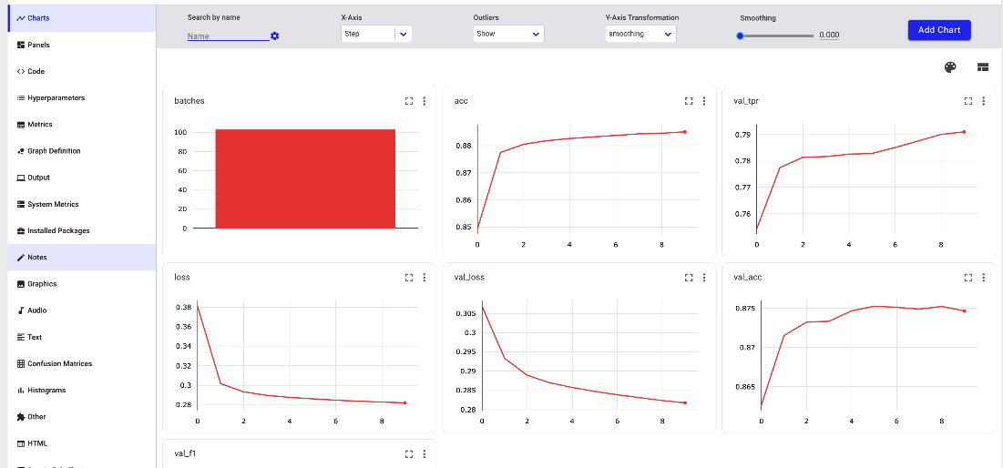
Figure 9.5 – An example of the output of the monitor() method

Each graph shows how a single metric evolves during the training phase.

We have just reviewed the main concepts behind Spark NLP and how to integrate it with Comet. Now, it is time to practice. Let’s start by setting up the environment to work with Spark NLP.

Setting up the environment for Spark NLP

Since Spark NLP runs on Apache Spark, you need to first set up Apache Spark to make Spark NLP work properly. Apache Spark requires Java to run properly; thus, you also need to install Java. Optionally, you can install Scala, another programming language.

To install Spark NLP, you should install the following frameworks and libraries:

• Python
• Java
• Scala (optional)
• Apache Spark
• PySpark and Spark NLP

We have already installed Python following the procedure described in the Technical requirements section, so we can start installing the software from the second step, Java.

Installing Java

Spark NLP is built at the top of Apache Spark, which can be installed on any operating system supporting Java. Apache Spark requires Java 8 to work properly:

1. To verify whether Java is already installed on your computer, as well as its current version, you can open a terminal and run the following command:

   Java –version

If Java is already installed, the command should return something similar to the following output:

openjdk version "1.8.0_322"

OpenJDK Runtime Environment (build 1.8.0_322-bre_2022_02_28_15_01-b00)

OpenJDK 64-Bit Server VM (build 25.322-b00, mixed mode)

The second digit after the version keyword indicates the current Java version, which is 8 in this case.

2. If Java is not installed, you can download it either from the official Oracle website or from other open source websites, such as OpenJDK. In Ubuntu, you can install openjdk-8 as follows:

   sudo apt-get install openjdk-8-jre

In macOS, you can run the following command, provided that you have brew installed:

brew install openjdk@8

In all cases, including Windows, you can download Java 8 from the following link, https://java.com/en/download/, and then follow the wizard.

3. If Java is already installed but you do not have version 8, you can install it following the procedure described in step 2, and then you set the JAVA_HOME environment variable to the path to the Java 8 directory.
4. Run step 1 again to make sure that Java 8 is installed properly.

Once you have installed Java, you can move on to the next step, installing Scala.

Installing Scala (optional)

Scala is a programming language used in data processing, distributed computing, and web development. You can find more information about Scala on its official website, available at the following link: https://www.scala-lang.org/.

Apache Spark requires Scala 2.12 or 2.13 to work properly:

1. You can install Scala 2.12.15 following the procedure described at the following link: https://www.scala-lang.org/download/2.12.15.html.
2. To verify that you have installed Scala correctly, you can run the following command:

   scala -version

The command should return version 2.12.

Once you have installed Scala, you are ready to install Apache Spark.

Installing Apache Spark

You can download Apache Spark from its official website, available at the following link: https://spark.apache.org/downloads.html.

1. For the examples described in this chapter, we will use version 3.1.2, available at the following link https://archive.apache.org/dist/spark/spark-3.1.2/.
2. Once you have downloaded the package, you can extract it and place it wherever you want in your filesystem. Then, you should add the path to the bin directory contained in your spark directory to the PATH environment variable. In Unix systems, you can export the PATH variable by adding the following line of code to your .bashrc or .zprofile (or other similar files, depending on your shell) file:

   export PATH=$PATH:/path/to/spark/bin

The exact filename you should modify depends on the specific shell you are using.

3. You also need to export the SPARK_HOME environment variable with the path to your spark directory. In Unix systems, you can export the SPARK_HOME variable as follows:

   export SPARK_HOME="/path/to/spark"

You should add the previous line of code to your .bashrc file (or similar file).

Note

You may need to exit and enter again your terminal to make changes effective.

4. To test whether you have installed Apache Spark correctly or not, you can run the following command:

   spark-shell

You should see output similar to the following one:

Welcome to

      ____              __

     / __/__  ___ _____/ /__

    _ / _ / _ '/ __/  '_/

   /___/ .__/\_,_/_/ /_/\_   version 3.1.2

      /_/

Using Scala version 2.12.15 (OpenJDK 64-Bit Server VM, Java 1.8.0_322)

Type in expressions to have them evaluated.

Type :help for more information.

scala>

5. To exit the Apache Spark shell, you can use Ctrl + C.

Now that we have installed Apache Spark, we can move on to the final step, installing PySpark and Spark NLP.

Installing PySpark and Spark NLP

To install PySpark, you can run the following command:

pip install pyspark

To install Spark NLP, you can run the following command:

pip install spark-nlp

It may happen that some pretrained models of pipelines are available only for specific versions of Spark NLP. Therefore, you can create a virtual environment to contain a specific version of Spark NLP. You can proceed as follows:

1. Firstly, you create a new virtual environment:

   python3 -m venv /path/to/your/virtual/environment

2. Then, you activate it:

   cd /path/to/your/virtual/environment

   source bin/activate

3. Now, you can install the specific version of Spark NLP, as follows:

   pip install spark-nlp==x.y.z

Note

In the new virtual environment, you should also install all the required libraries to run your software. For example, if you use Jupyter to create your code, you should install and run it in your virtual environment.

Now that we have installed all the software required to run Spark NLP, let’s move on to a practical example.

Using NLP, from project setup to report building

In this section, you will implement a practical example that performs sentiment analysis of some text extracted from Twitter. This example compares a pretrained model and a custom model, showing the results in Comet.

The full code of the example described in this section is available at the following link: https://github.com/PacktPublishing/Comet-for-Data-Science/tree/main/09.

We will focus on the following aspects:

• Configuring the environment
• Loading the dataset
• Implementing a pretrained pipeline
• Logging results in Comet
• Using a custom pipeline
• Building the final report

Let’s start from the first point, configuring the environment.

Configuring the environment

Environment configuration involves the following two steps:

1. We initialize Spark NLP. We import and start the Spark NLP library as follows:

   import sparknlp

   spark = sparknlp.start()

Note

If you are writing you code in Jupyter, the previous command may fail because your kernel is not able to find the Apache Spark directory. To solve the problem, before calling sparknlp.start(), use the findspark Python library, as follows:

import findspark

findspark.init()

2. We initialize Comet. We import and initialize the Comet library, as follows:

   import comet_ml

   from sparknlp.logging.comet import CometLogger

   comet_ml.init()

   logger = CometLogger()

   logger.experiment.set_name('PretrainedModel')

We should have a .comet.config file, which contains our Comet credentials and is located in the same directory as the working directory, as described in Chapter 1, An Overview of Comet.

Now that we have configured the environment, we can move to the next step, loading the dataset.

Loading the dataset

As a use case, you will use the Disneyland Reviews dataset, available on Kaggle at the following link, https://www.kaggle.com/datasets/arushchillar/disneyland-reviews, and released under the CC0: Public Domain license. The dataset contains 42,656 reviews of three Disneyland branches (Paris, California, and Hong Kong) posted by visitors on Tripadvisor. For each review, it also provides the rating, which ranges from 1 (totally unsatisfied) to 5 (satisfied). We group ratings into two categories: positive if the rating is greater than 2, and negative otherwise. For simplicity, we assume that a positive rating also corresponds to a positive sentiment within the text review, and a negative rating also corresponds to a negative sentiment within the text review.

The following table shows the first two rows of the dataset:

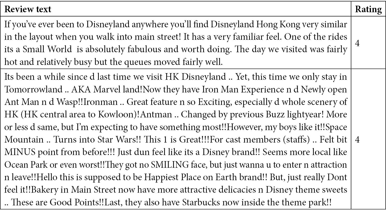
Figure 9.6 – Extracts from the Disneyland Reviews dataset

The dataset has many columns; from them, we will use the following: Review_Text, which contains the text, and Rating, which contains the rating and which we will use as a sentiment.

We perform the following steps to load the dataset as a pyspark DataFrame:

1. Firstly, we load the dataset:

   from pyspark.sql.functions import when, col

   df=spark.read.format("csv").option("header", "true").load("source/DisneylandReviews.csv")

We use the format() function provided by the Spark NLP library to load the package, as well as the option header, set to true to read the CSV header.

2. Then, we group rows as follows:

   df = df.withColumn("sentiment", when(col("Rating") > 2, "positive").otherwise("negative"))

We mark rows with a Rating value greater than 2 as positive, and those with a Rating value fewer or equal to 2 as negative.

The previous operation is required by the pretrained model that we will use.

Now that we have loaded the dataset, we can move on to the next step, implementing a pretrained pipeline.

Implementing a pretrained pipeline

The first pipeline we will implement uses the pretrained model named ViveknSentimentModel, provided by Spark NLP. You can find more information about the pretrained model and how to use it at the following link: https://nlp.johnsnowlabs.com/2021/11/22/sentiment_vivekn_en.html.

1. Firstly, we import all the required packages:

   from sparknlp.base import *

   from sparknlp.annotator import *

   from pyspark.ml import Pipeline

2. Now, we implement the Spark pipeline with the following five stages:

   document = DocumentAssembler()

       .setInputCol("Review_Text")

       .setOutputCol("document")

   token = Tokenizer()

       .setInputCols(["document"])

       .setOutputCol("token")

   normalizer = Normalizer()

       .setInputCols(["token"])

       .setOutputCol("normal")

   vivekn =  ViveknSentimentModel.pretrained()

       .setInputCols(["document", "normal"])

       .setOutputCol("result_sentiment")

   finisher = Finisher()

       .setInputCols(["result_sentiment"])

       .setOutputCols("final_sentiment")

The pipeline stages include the document assembler, the tokenizer, the normalizer, the pretrained model of the Vivekn sentiment model, and the finisher.

3. We create the pipeline:

   pipeline = Pipeline().setStages([document, token, normalizer, vivekn, finisher])

4. Now, we fit the pipeline with the text:

   X = df.select('Review_Text').toDF('Review_Text')

   pipelineModel = pipeline.fit(X)

We have built an auxiliary variable called X, which contains only the text.

5. Finally, we calculate the results:

   result = pipelineModel.transform(X)

Now that we have trained the pipeline, we are ready to log the results in Comet.

Logging results in Comet

In Comet, we can now log the evaluation results:

1. To perform this operation, we need to map the results produced by the pipeline with the original sentiment labels, as shown in the following piece of code:

   df_tot = df.join(result, on=["Review_Text"])

We have built a new spark DataFrame, called df_tot, which has the following structure:

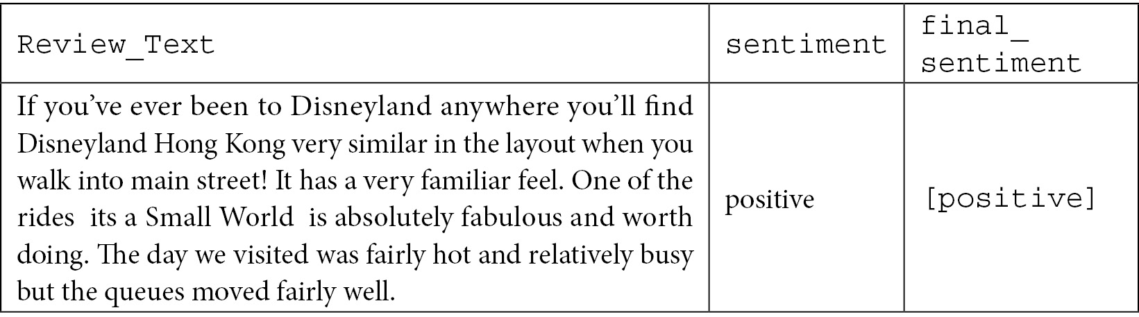
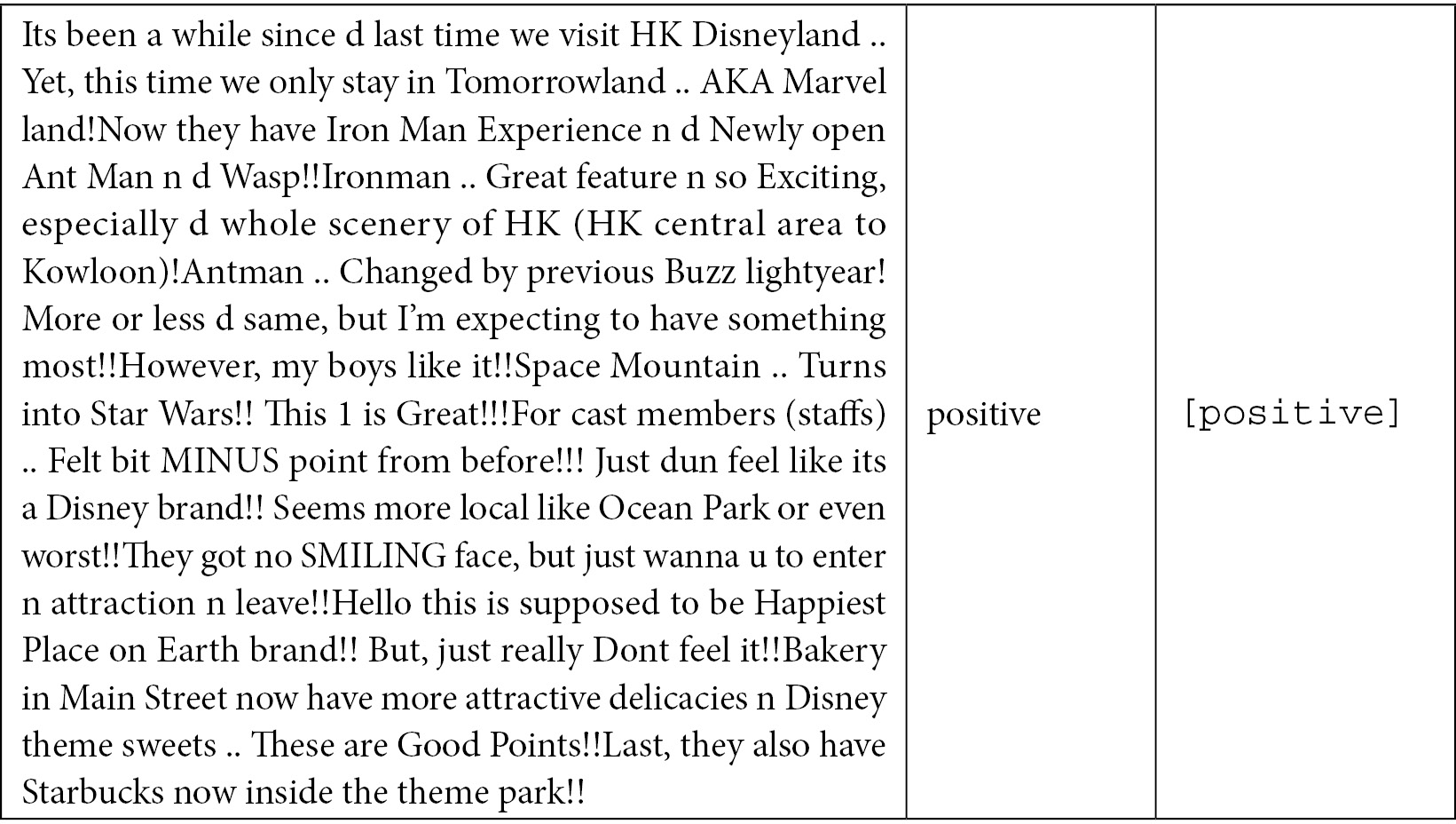
Figure 9.7 – The merged DataFrame, with both a true sentiment (sentiment) and a predicted sentiment (final_sentiment)

2. To log the results in Comet, we need to convert the Spark DataFrame into a pandas DataFrame, as shown in the following piece of code:

   pandas_df = df_tot.toPandas()

3. We need to convert to strings the lists contained in the final_sentiment columns:

   pandas_df['predicted_sentiment'] = [','.join(map(str, l)) for l in pandas_df['final_sentiment']]

We have built a new column, called predicted_sentiment, which stores the cleaned version of final_sentiment. We will use predicted_sentiment for further analysis.

4. We use the classification_report() function provided by scikit-learn to calculate precision, recall, and the F1 score:

   from sklearn.metrics import classification_report

   report = classification_report(pandas_df['sentiment'], pandas_df['predicted_sentiment'], output_dict=True, labels=['positive', 'negative'])

5. We log the results in Comet:

   for key, value in report.items():

       if key!='accuracy':

           logger.log_metrics(value,prefix=key)

       else:

           logger.log_metrics({"accuracy": value})

After running the experiment, you should see the results in Comet, as shown in the following figure:

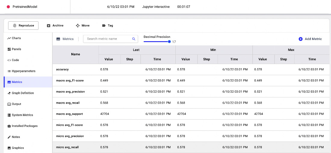
Figure 9.8 – The evaluation metrics of the pretrained model in Comet

Now that we have logged the results of the first pipeline in Comet, we can move on to the second pipeline.

Using a custom pipeline

The custom pipeline trains a custom model, based on the ViveknSentimentApproach class. The pipeline contains the same stages as the previous examples, with the exception of the model:

vivekn_custom = ViveknSentimentApproach() 

    .setInputCols(["document", "normal"]) 

    .setSentimentCol("sentiment") 

    .setOutputCol("result_sentiment")

While in the previous example the model was already trained, this time you need to train it.

To perform training, you can implement the following steps:

1. Firstly, we split the dataset into training and test sets, as described in the following piece of code:

   (training_set, test_set) = df.randomSplit([0.8, 0.2])

   X_train = training_set.select('Review_Text', 'sentiment').toDF('Review_Text', 'sentiment')

   X_test = test_set.select('Review_Text', 'sentiment').toDF('Review_Tex', 'sentiment')

We have reserved 80% of the samples for the training set and the remaining 20% for the test set.

2. Then, we train the pipeline on the training set:

   pipelineModel = pipeline.fit(X_train)

3. Finally, we calculate predictions on the test set:

   result = pipelineModel.transform(X_test)

Once you have trained the model and calculated the predictions for the test set, you can log the results in Comet, as you did in the previous example. Since ViveknSentimentApproach does not implement the setOutputLogsPath() method, we cannot monitor the training process in Comet.

Now that we have built the custom model and evaluated its performance, we can proceed with the final step, building the final report.

Building the final report

Now, you are ready to build the final report. In this example, we will build a simple report with a comparison between the two models. As a further exercise, you can improve them by applying the concepts learned in Chapter 5, Building a Narrative in Comet. You will create a report with a section containing the comparison between the calculated performance metrics in the two models.

We perform the following two steps:

• Building the panels
• Building the report

Let’s start from the first step, building the panels.

Building the panel

We implement the following panels:

• A bar chart, for the performance metrics at the macro level, and another for the performance metrics at the micro level
• A parallel coordinates chart to compare the different performance metrics, calculated for each target class (positive and negative sentiment)
• A project summary, which contains all the performance metrics for both the experiments in a tabular form

To build the first bar chart for metrics at the macro level, you can follow the following steps:

1. From the Comet project main dashboard, select the Panels tab, and then Add | New Panel | BUILT-IN | Bar Chart | Add.
2. In the Y-Axis input textbox, select the accuracy.
3. Click on the Add field button, and select macro avg_f1_score.
4. Repeat the previous two steps to also add macro avg_precision and macro avg_recall.
5. Click on the Done button. You should see a graph similar to the one shown in the following figure:

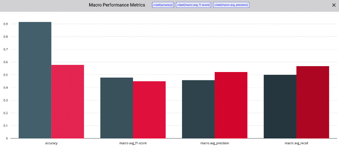
Figure 9.9 – The bar chart panel for the macro performance metrics

To build the parallel coordinates chart, you can perform the following steps:

1. From the Comet project main dashboard, select the Panels tab, and then Add | New Panel | BUILT-IN | Parallel Coordinates Chart | Add.
2. In the Target Variable input textbox, select the accuracy.
3. In the Y-Axis input textbox, you can add as many metrics as you want. In our example, we add the following metrics: positive_precision, positive_recall, negative_precision, and negative_recall.
4. Click on the Done button. You should see a graph similar to the one shown in the following figure:

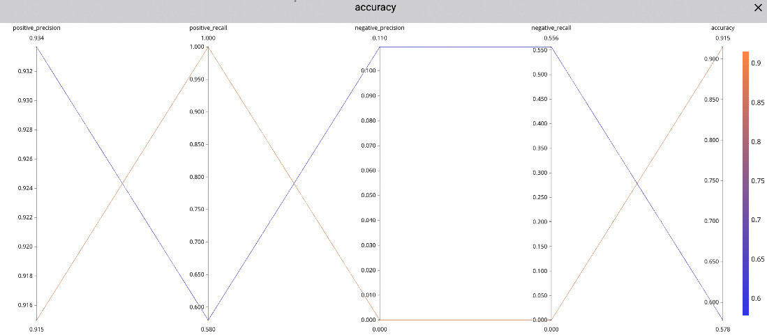
Figure 9.10 – The parallel coordinates chart

5. To build the Project Summary panel, select the Panels tab, and then Add | New Panel | FEATURED | Project Summary | Add | Done. The produced panel should be similar to the one shown in the following figure:

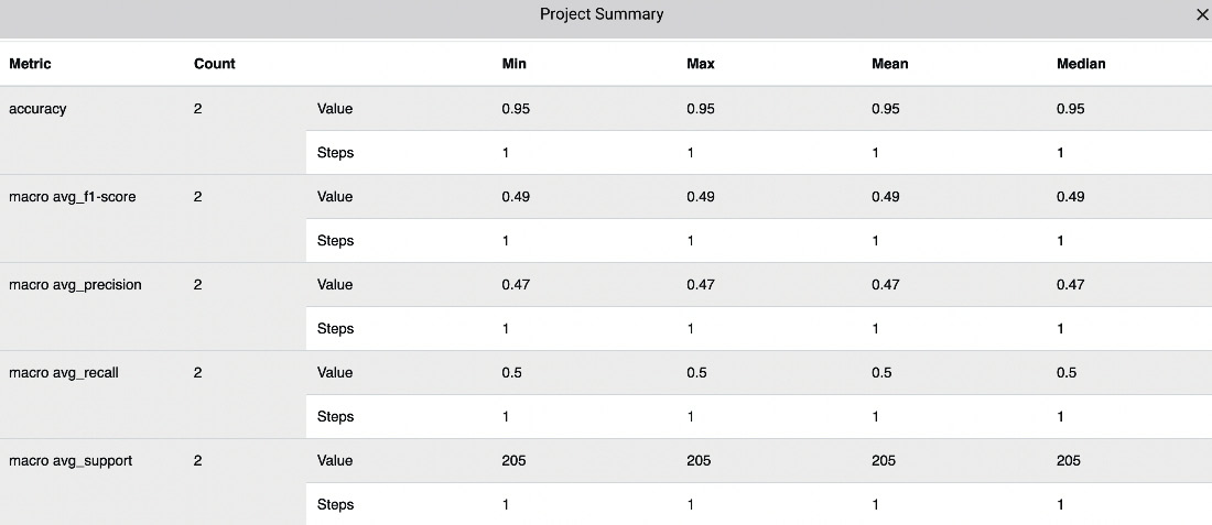
Figure 9.11 – The Project Summary panel

Now that we have built the panels, we can add them to the report. Thus, we can move on to the final step, building the report.

Building the report

To create the report, in the Comet dashboard, perform the following steps:

1. Click on the Panels tab, and then select Add | Add to Report | New Report.
2. A new report appears with the previously created panels.
3. You can customize the size of each chart in the panel by selecting the Edit Layout button and then adjusting the layout of each chart with the mouse.
4. You can customize your report with the title, descriptions, and so on.
5. Finally, click on the Save button.

The following figure shows a snapshot of part of the final report:

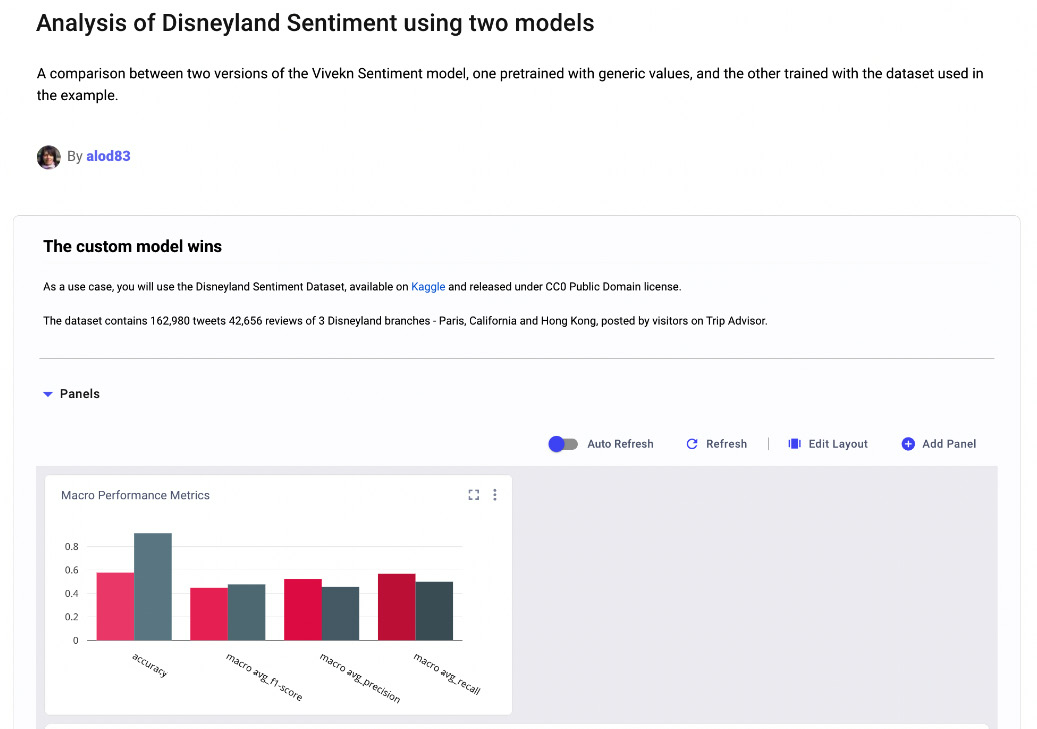
Figure 9.12 – A snapshot of the final report

You can see the full report at https://www.comet.ml/packt/spark-nlp/reports/analysis-of-dysneyland-sentiment-using-two-models, while the full project in Comet is available at the following link: https://www.comet.ml/packt/spark-nlp/.

Summary

We just completed the journey to build an NLP model in Spark NLP and track it in Comet!

Throughout this chapter, we described some general concepts regarding NLP, including the basic NLP workflow, how you can classify NLP tools, and the main NLP challenges. In addition, you have seen the main structure of the Spark NLP package and how to set up the environment to make it work. We also illustrated some important concepts, such as annotators and pipelines.

In the last part of the chapter, you implemented a practical use case that showed you how to track an NLP experiment in Comet, as well as how to build a report with the results of the experiment.

In the next chapter, we will review the basic concepts related to deep learning and how to perform it in Comet.

Further reading

• Kedia, A., and Rasu, M. (2020). Hands-On Python Natural Language Processing: Explore tools and techniques to analyze and process text with a view to building real-world NLP applications. Packt Publishing Ltd.
• Thomas, A. (2020). Natural Language Processing with Spark NLP: Learning to Understand Text at Scale. O’Reilly Media, Inc.