Chapter 8: Comet for Machine Learning

Artificial intelligence (AI) is the ability of a computer to perform operations and tasks that are usually done by humans. AI includes different subfields, such as machine learning, natural language processing, deep learning, and time series analysis. In this chapter, we will focus on machine learning, and in the following ones, you will review other subfields of AI, including natural language processing (Chapter 9,Comet for Natural Language Processing), deep learning (Chapter 10, Comet for Deep Learning), and time series analysis (Chapter 11, Comet for Time Series Analysis).

Machine learning aims at using computational algorithms to transform data into usable models. In other words, machine learning tries to build models that learn from data. You can use machine learning algorithms for different purposes and in different domains, such as describing a phenomenon, predicting future values, or detecting anomalies in a phenomenon under investigation. You have already learned some concepts about machine learning in previous chapters, including exploratory data analysis (Chapter 2, Exploratory Data Analysis in Comet) and model evaluation (Chapter 3, Model Evaluation in Comet). In this chapter, we will focus on model training, which involves building the correct model to represent a given phenomenon.

In recent years, different open source libraries and tools were available to build machine learning models. In this chapter, we will focus on scikit-learn and XG-Boost. You should already be familiar with scikit-learn, since you have already used it in the examples described in previous chapters. You have also learned how to integrate Comet with scikit-learn. In this chapter, you will implement a complete use case, which will permit you to implement a complete machine learning pipeline in Comet.

The chapter is organized as follows:

• Introducing machine learning
• Reviewing the main machine learning models
• Reviewing the scikit-learn package
• Building a machine learning project from setup to report

Before moving on to the first step, let’s see the technical requirements to run the software used in this chapter.

Technical requirements

We will run all the experiments and code in this chapter using Python 3.8. You can download it from the official website at https://www.python.org/downloads/ and choose version 3.8.

The examples described in this chapter use the following Python packages:

• comet-ml 3.23.0
• matplotlib 3.4.3
• numpy 1.19.5
• pandas 1.3.4
• scikit-learn 1.0
• shap 0.40.0

We have already described the first five packages and how to install them in Chapter 1, An Overview of Comet. So please refer back to that for further details on installation.

shap

shap is a Python package that permits you to calculate the Shapley value and plot some related graphs. To install the shap package, you can run the following command in a terminal:

pip install shap

For more details on the shap package, you can refer to its official documentation, available at the following link: https://shap-lrjball.readthedocs.io/en/latest/index.html.

Now that you have installed all of the software needed in this chapter, let’s move on to how to use Comet for machine learning, starting with reviewing some basic concepts on machine learning.

Introducing machine learning

Machine learning is a subfield of AI that aims to build models that automatically learn from data. You can use these models for different purposes, such as describing a particular phenomenon, predicting future values, or detecting anomalies in an observed phenomenon. Machine learning has become very popular in recent years thanks to the spread of huge quantities of data that derive from different sources, such as social media, open data, sensors, and so on.

The section is organized as follows:

• Exploring the machine learning workflow
• Classifying machine learning systems
• Exploring machine learning challenges
• Explaining machine learning models

Let’s start with the first step: exploring the machine learning workflow.

Exploring the machine learning workflow

The following figure shows the simplest machine learning workflow:

Figure 8.1 – The simplest machine learning workflow

Provided that you already know the problem you want to solve, there are four steps:

1. Data preprocessing: You prepare your data by performing all the cleaning operations, including dealing with missing values and anomalies, normalization, standardization, and dropping duplicates. In this phase, you also split your data into training, dev, and test sets.
2. Feature engineering: You choose the set of features in your data to send as input to the model.
3. Model training: You train your model on the training set, with a focus on tuning model parameters (hyperparameter tuning). In this phase, usually, you apply cross-validation.
4. Model evaluation: You evaluate the performance of your model on the dev set by choosing the set of evaluation metrics. You have already learned how to perform the model evaluation in Chapter 3, Model Evaluation in Comet.

We will review how scikit-learn permits you to implement the preceding steps later in this chapter in the Reviewing the scikit-learn package section.

Now that you have reviewed the simplest machine learning workflow, we can move on to the next step: classifying machine learning systems.

Classifying machine learning systems

You can classify machine learning systems based on the following three main criteria:

• The nature of the problem to solve (supervised, unsupervised, semi-supervised, and reinforcement learning)
• The learning technique used (batch and online learning)
• The internal nature of the algorithm (instance-based and model-based learning)

Let’s investigate each criterion separately, starting with the first one: the nature of the problem to solve.

The nature of the problem to solve

In Chapter 3, Model Evaluation in Comet, you already encountered two types of machine learning models: supervised learning and unsupervised learning. There is an additional technique, called semi-supervised learning. The following are the main objectives of each technique:

• The main objective of supervised learning is to learn the mapping function between the input and the output values. In supervised learning, for each input value in the training set, you also know the output value, and the objective is to build a model that learns the mapping function from input to output. Output values are also known as labels. Once you have built the model, you can use it to predict the labels of new and unseen input values. There are two types of supervised learning: classification and regression. You reviewed the basic concepts behind classification and regression in Chapter 3, Model Evaluation in Comet.
• The main objective of unsupervised learning is to group input values based on some criteria of similarity. The main types of unsupervised learning include clustering, anomaly detection, and dimensionality reduction. You reviewed the basic concepts behind clustering in Chapter 3. We will review the other two types of unsupervised learning in the Reviewing the scikit-learn package section.
• Semi-supervised learning has the same objective as supervised learning. However, in semi-supervised learning, only a subset of input values is labeled, so the model should combine both supervised and unsupervised learning techniques to predict the output value.

Now that you have learned how to classify machine learning models based on the nature of the problem to solve, we can move on to the next criterion: the learning technique used.

The learning technique used

If you consider the learning technique used, you can classify machine learning systems into the following two types:

• Batch learning systems: You perform the training process offline, just once. You cannot update the model on the fly. Usually, this technique requires a lot of computational resources.
• Online learning systems: You can train the system incrementally. Usually, in each step, you feed the system with a small batch of data, also called mini-batches. You can use this technique when you have a continuous flow of data that you can feed to the model.

Now that you have learned how to classify machine learning models based on the learning technique used, we can move on to the final criterion: the internal nature of the algorithm.

The internal nature of the algorithm

Depending on the internal nature of the algorithm, you can have the following types of learning:

• Instance-based learning: The algorithm learns from data in the training set to find a data pattern that can be used for future predictions. In practice, the algorithm predicts the output for new samples based on similarity with the data in the training set. This type of algorithm preserves the original training set that is used at each prediction. The main drawback of this category of algorithms is that the model size could be huge if the training set size is huge. The k-nearest neighbor classifier, for example, falls in this category of algorithms.
• Model-based learning: The algorithm builds a mathematical model that approximates the data in the training set. Once the algorithm has built the model, the original dataset can be deleted. The decision tree classifier is an example of model-based learning. The main drawback of this category of algorithms is that you can hardly apply online learning in this case.

Now that you have briefly reviewed how you can classify machine learning systems, we can move on to the next step: exploring machine learning challenges.

Exploring machine learning challenges

When you build a machine learning model, you may encounter different challenges and issues that can be grouped into the following two big families:

• Data challenges
• Model challenges

Let’s investigate each family separately, starting with the first: data challenges.

Data challenges

The following table shows the most common data challenges:

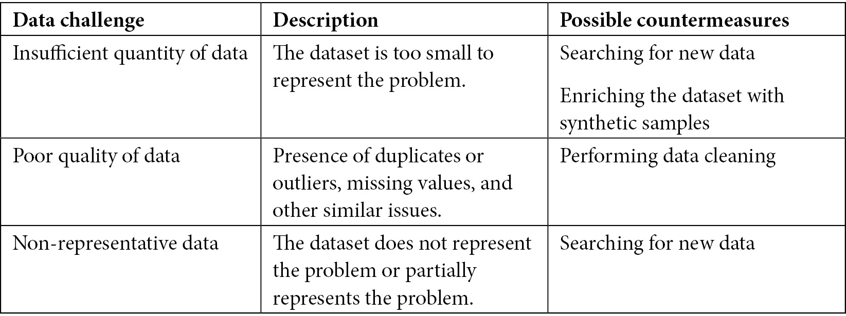
Figure 8.2 – The most common data challenges

The table also describes some possible countermeasures against the described challenges. For example, if you have an insufficient quantity of data, you may search for new data, or enrich the dataset with new data or even with synthetic data.

Model challenges

The following table shows the most common model challenges:

Figure 8.3 – The most common model challenges

When compared to data challenges, model challenges are more complicated to solve because they depend on the specific model you are using. The best way to deal with model challenges is to try different models and select the one with the best performance.

Now that you have briefly reviewed the main machine learning challenges, we can move on to the next step: explaining machine learning models.

Explaining machine learning models

Usually, you see a machine learning model as a black box that takes some features as input and produces an output (also called a target). What happens inside the black box depends on the specific algorithm you are using. To understand how each feature contributes to the output in the model, you can use different techniques. In this section, you will learn about SHAP.

The SHapley Additive exPlanations (SHAP) algorithm uses the concept of the Shapley value, which derives from game theory where you have a game and many players. In machine learning, the game is the output of the model and the players are the input features. The Shapley value calculates the contribution of each player to the game. In other words, it calculates the contribution of each input feature to build the final prediction of the model.

For each observation in the training set, you have a different game, thus you can use the Shapley value to analyze a single output each time.

Python provides a package, named shap, to calculate the Shapley value and to plot some useful graphs, which help you understand the contribution of each input feature to the output. The shap library is fully integrated with Comet.

In the remainder of this section, you will learn the following topics:

• Using the shap library
• Integrating the shap library in Comet

Let’s start with the first topic: using the shap library.

Using the shap library

To calculate the Shapley value, you need to perform the following steps:

1. First, you should create an Explainer object. The shap library provides different types of Explainer objects, including, but not limited to, TreeExplainer, GradientExplainer, DeepExplainer, and so on. Each Explainer is related to the specific implemented algorithm. The Explainer object receives as input the trained model, as shown in the following piece of code:

   import shap

   shap.initjs()

   explainer = TreeExplainer(model)

You import the library, then you need to call the initjs() function, and, finally, you can build the Explainer object. In this case, we have created a TreeExplainer.

2. Once you have created the object, you can calculate the Shapley value for a single observation or many observations as follows:

   shap_values = explainer.shap_values(X)

If the model represents a classification task, the shap_values() method returns a list containing the Shapley values for each target class.

3. Using the calculated Shapley values, you can plot different graphs, including bar plots, decision plots, summary plots, and so on. For a complete list of descriptions of the available plots, you can refer to the shap official documentation, available at the following link: https://shap.readthedocs.io/en/latest/api_examples.html#plots.

Now that you have seen an overview of the shap package, we can investigate how to integrate the graphs produced with shap in Comet.

Integrating the shap library in Comet

To integrate one or more graphs produced with the shap library in Comet, you can perform the following steps:

1. Import the Comet library before importing shap, as shown in the following piece of code:

   from comet_ml import Experiment

   import shap

   shap.initjs()

2. Create a Comet Experiment and then an Explainer object as follows:

   experiment = Experiment()

   explainer = shap.Explainer()

3. Use any of the functions provided by shap to plot a graph as follows:

   shap_values = explainer.shap_values(X_test)

   shap.summary_plot(shap_values, X_test)

The preceding code plots a summary plot for the Shapley values passed as input argument. The graph will be automatically logged in Comet under the Graphics section.

Now that you have learned some basic concepts regarding the shap library and how to integrate it in Comet, we can move on to the next step: a review of the main machine learning models.

Reviewing the main machine learning models

A machine learning model is an algorithm that can make predictions for some unseen data based on what it has learned from some training data. As already discussed in the preceding section, you can distinguish machine learning models into two categories, which depend on the specific task you want to solve: supervised models and unsupervised models.

Many machine learning models exist in the literature. In this section, you will review the most popular models used to perform supervised learning and unsupervised learning. We will focus on the following models in detail:

• Supervised learning
• Unsupervised learning

In the remainder of the section, you will review an introduction to the most popular machine learning models. For more details, you can read the books proposed in the Further reading section. Let’s start with the first category of models: supervised learning.

Supervised learning

A supervised algorithm receives a sample as input, performs some computations, and returns a predicted value as output. If the output is a continuous variable, you will have a regression problem, but if the output is a discrete variable, such as a class label, you will have a classification problem.

The following supervised algorithms are some of the most popular ones:

• Linear regression: The algorithm searches for a line that best fits the input samples.
  • Logistic regression: The algorithm uses the logistic unit to model the input samples. Contrary to what the name might suggest, logistic regression is used to solve classification problems.
  • Support vector machines (SVM): The algorithm searches for a hyperplane that groups training data by common features.
  • Naive Bayes: The algorithm assumes that the input features are independent. It uses Bayes’s theorem to produce results.
  • Decision trees: The algorithm uses a tree to predict the output. Each node of the tree represents an input feature, whereas the leaves of the tree represent the possible outputs.
  • K-nearest neighbors: The algorithm uses proximity to group the input samples and predict the output.
  • Random forest: The algorithm uses multiple trees to predict the output.

After a brief overview of the most popular algorithms for supervised learning, we can move on to reviewing the algorithms for unsupervised learning.

Unsupervised learning

An unsupervised algorithm aims at grouping similar objects. A typical example of unsupervised learning is clustering.

One of the most popular algorithms for unsupervised learning is k-means, which tries to split the dataset into k non-overlapping sub-groups.

Now that you have learned the main machine learning models, we can move on to the next topic: a review of the scikit-learn package.

Reviewing the scikit-learn package

scikit-learn is a very popular Python package for machine learning. You have already encountered this package in previous chapters. In particular, you have focused on some examples using supervised learning and model selection. However, the scikit-learn package also provides other classes and methods, as shown in the following figure:

Figure 8.4 – An overview of the scikit-learn package

The package is divided into the following subpackages:

• Preprocessing
• Dimensionality reduction
• Model selection
• Supervised learning
• Unsupervised learning

Let’s investigate each subpackage briefly, starting with the first one: preprocessing. For a more in-depth analysis of each subpackage, you can refer to the Further reading section at the end of this chapter.

Preprocessing

Preprocessing contains all of the classes and methods that permit us to manipulate the dataset before giving it as input to a machine learning model. You can also use the methods provided by pandas as an alternative to almost all of the classes and methods provided in the preprocessing subpackage.

Preprocessing includes classes for the following:

• Feature scaling to perform data standardization and normalization
• Feature binarization to convert features into binary values
• Feature encoding to convert categorical features into numerical values
• Non-linear transformations to apply non-linear transformations to features, such as power transform
• Other classes to perform other specific transformations

Now that you have briefly reviewed the most important classes provided by the preprocessing package, we can analyze the next subpackage: dimensionality reduction.

Dimensionality reduction

Dimensionality reduction is a technique that reduces the number of input features from a high-dimensional space to a low-dimensional space.

Dimensionality reduction is especially useful when you have millions of input features, which could slow down the model training process. However, although the use of dimensionality reduction techniques speeds up the training process, it still leads to the loss of information.

Dimensionality reduction is also useful for data visualization because if you reduce the number of features down to two or three, you can easily plot them and perform a visual exploratory data analysis.

Figure 8.4 shows the most important techniques provided by scikit-learn to perform dimensionality reduction. Among them, the most popular technique is principal component analysis (PCA). The following piece of code shows how to implement PCA in scikit-learn:

from sklearn.decomposition import PCA

pca = PCA(n_components=2)

X_reduced = pca.fit_transform(X)

We have used the PCA class, which receives as input the final dimensionality of features (n_components). To get the reduced feature dataset, you should call the fit_transform() method on the input features (X).

Now that you have seen an overview of the dimensionality reduction package, we can analyze the next subpackage: model selection.

Model selection

Model selection includes the following techniques that help you select the best model for your problem:

• Cross-validation
• Hyperparameter tuning
• Metrics and curves

Let’s investigate the first two techniques, starting with cross-validation.

Metrics and curves

You remember that model selection also includes the study of metrics and curves for model evaluation. We reviewed this aspect in Chapter 3, Model Evaluation in Comet, so you can refer to that for further details.

Cross-validation

Cross-validation is a technique that permits you to calculate the performance of a machine learning algorithm on a dataset. k-fold cross-validation is one of the most popular techniques to perform cross-validation. It divides the datasets in k non-overlapping folds, then it fits k models and calculates the performance of each one. At each iteration, it uses k-1 folds as the training set and the remaining fold as the test set, as shown in the following figure:

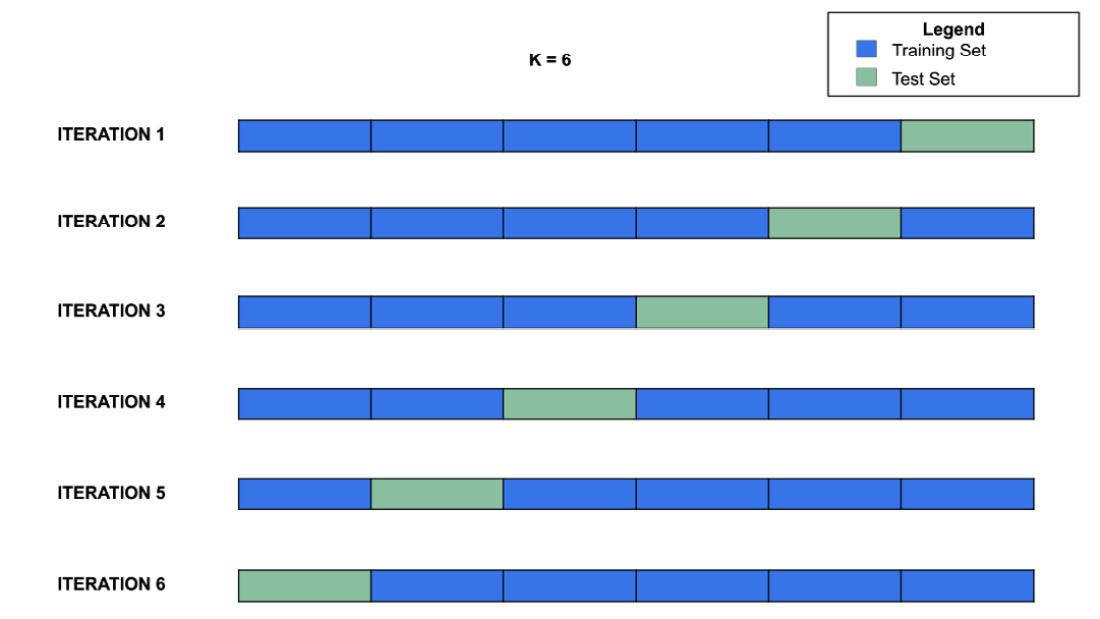
Figure 8.5 – k-fold cross-validation with k = 6

The figure shows how the k-fold cross-validation algorithm builds the training and test sets at each iteration in the case of k = 6. A common value for k is 10, but, usually, you should run different tests to calculate the most appropriate value for k. In the last section of this chapter, you will learn a practical strategy to calculate the best value for k in a practical example.

The performance of the model is calculated as the average value of the results of the k models.

scikit-learn provides the KFold class to perform basic k-fold cross-validation. This class receives the following parameters as input:

• n_splits: The number of folds, representing the parameter k.
• shuffle: A Boolean representing whether or not to shuffle the dataset before splitting it into folds.
• random_state: If shuffle is True, random_state affects how shuffle is performed.

scikit-learn also provides other classes to perform cross-validation, such as StratifiedKFold and GroupKFold. For more details on them, you can refer to the scikit-learn official documentation, available at the following link: https://scikit-learn.org/stable/modules/cross_validation.html.

Now that you have reviewed the basic concepts behind cross-validation, we can move on to the next point: hyperparameter tuning.

Hyperparameter tuning

Hyperparameter tuning permits you to search for the best parameters of a specific machine learning algorithm. Usually, you perform hyperparameter tuning in combination with cross-validation. You have already learned how to perform hyperparameter tuning in Comet in Chapter 4, Workspaces, Projects, Experiments, and Models. In this chapter, you will review the classes and methods provided by scikit-learn to perform hyperparameter tuning.

In general, you define a grid of parameters to test and you pass it as input of an algorithm, which fits as many models as the different combinations of parameters. Finally, the algorithm calculates the model with the best performance and returns it as the best model.

scikit-learn implements different algorithms to perform hyperparameter tuning, including, but not limited to, the following ones:

• GridSearchCV: The algorithm tests all of the possible combinations of parameters.
• RandomizedSearchCV: The algorithm performs a randomized search over parameters.
• HalvingGridSearchCV: The algorithm first tests all of the parameters on a small dataset, then iteratively discards the parameters with the lowest performance and continues the tests on the remaining parameters by adding new samples to the dataset.

In the last section of this chapter, you will see a practical example that uses the GridSearchCV algorithm. For more details on how to use the other algorithms, you can refer to the scikit-learn official documentation, available at the following link: https://scikit-learn.org/stable/modules/classes.html#module-sklearn.model_selection.

Now that you have reviewed the basic concepts behind hyperparameter tuning, we can move on to the next point: supervised and unsupervised learning.

Supervised and unsupervised learning

scikit-learn implements the most popular algorithms to perform both supervised and unsupervised learning. In all cases, to implement a model, you should perform the following steps:

1. Create the model as follows:

   model = MyModel()

You should replace the MyModel() class with the specific class provided by scikit-learn, such as KNeighborsClassifier or LinearRegression.

2. Fit the model with the training set as follows:

   model.fit(X_train, y_train)

3. Use the trained model to predict the output for unseen inputs as follows:

   y_pred = model.predict(X_test)

The preceding steps describe the very basic operations you should perform to build a machine learning model. In the following section of this chapter, you will implement a more complex example that also considers cross-validation and hyperparameter tuning as well as the integration with Comet. So, let’s move on to this practical example.

Building a machine learning project from setup to report

In this section, you will further improve the practical example of diamond cuts described in Chapter 3, Model Evaluation in Comet, and deployed in Chapter 6, Integrating Comet into DevOps. In this chapter, you will focus on the following aspects:

• Reviewing the scenario
• Selecting the best model
• Calculating the SHAP value
• Building the final report

Let’s start with the first step: reviewing the scenario.

Reviewing the scenario

As our use case, we will use the diamonds dataset provided by ggplot2 under the MIT licenses (https://ggplot2.tidyverse.org/reference/diamonds.html) and available on Kaggle as a CSV file (https://www.kaggle.com/shivam2503/diamonds). With respect to the original version, already described in Figure 3.3 in Chapter 3, we use the cleaned version produced in the same chapter and shown in the following figure:

Figure 8.6 – The cleaned version of the diamonds dataset

The dataset contains 53,940 rows and 10 columns. The objective of this scenario is to build a classification model that, when given a set of input features, predicts the target category (Gold, Silver). We suppose that the input features are stored in a variable called X and the target in a variable called y, as shown in the following piece of code:

X = df.drop("target", axis = 1)

y = df["target"]

We have supposed that the dataset is loaded as a pandas DataFrame. We preprocess the dataset by encoding labels and scaling numeric values. For more details on how to perform these operations, you can refer to Chapter 3.

Now that you have reviewed the employed dataset, we can move on to the next step: selecting the best model.

Selecting the best model

To select the best model, we compare the performance of the following four classification algorithms, as already described in Chapter 3, Model Evaluation in Comet: random forest, decision tree, Gaussian Naive Bayes, and k-nearest neighbors. For each algorithm, we search for the optimal model by performing the following steps:

• Searching for the best number of folds for cross-validation
• Performing hyperparameters tuning with cross-validation

We will build a Comet experiment for each test performed. We use accuracy as a metric to select the best model.

Let’s start with the first step: searching for the best number of folds for cross-validation.

Searching for the best number of folds for cross-validation

To get familiar with cross-validation, we first run a simple experiment, which compares the performance of each algorithm with and without the use of cross-validation, with a fixed number of folds (10). When you build the model without cross-validation, you should use the train/test splitting operation to fit the model on the training set and evaluate it on the test set. On the other hand, if you build the model with cross-validation, you can use the whole dataset because cross-validation already performs train/test splitting. Perform the following steps to find the best number of folds for cross-validation:

1. We split the dataset into training and test sets as follows:

   from sklearn.model_selection import train_test_split

   X_train, X_test, y_train, y_test = train_test_split(X, y, test_size=0.10, random_state=42)

We reserve 10% of records for the test set and the remaining for the training set.

2. We define a function, named run_experiment(), that builds an Experiment in Comet and then logs in Comet the accuracy of the model passed as an argument, either when using cross-validation or not, as follows:

   from sklearn.model_selection import KFold

   from sklearn.model_selection import cross_val_score

   from sklearn.metrics import accuracy_score

   import numpy as np

   def run_experiment(ModelClass, name, n_splits):

       experiment = Experiment()

       experiment.set_name(name)

       experiment.add_tag(name)

       

       cv = KFold(n_splits=n_splits, random_state=1, shuffle=True)

       model = ModelClass()

       # calculating accuracy with KFold

       scores = cross_val_score(model, X, y, scoring='accuracy', cv=cv)

       experiment.log_metric('accuracy-cv', np.mean(scores))

       

       # calculating accuracy without KFold

       model.fit(X_train, y_train)

       y_pred = model.predict(X_test)

       experiment.log_metric('accuracy', accuracy_score(y_test, y_pred))

We use KFold() with the shuffle=True parameter to perform an initial shuffle of the dataset. To calculate the accuracy in the case of k-fold, we use the cross_val_score() function. We log the accuracy obtained from cross-validation as accuracy-csv and the accuracy obtained without cross-validation as accuracy.

3. Now we can run the experiments simply by calling the run_experiment() function for the four algorithms as follows:

   from sklearn.ensemble import RandomForestClassifier

   from sklearn.tree import DecisionTreeClassifier

   from sklearn.naive_bayes import GaussianNB

   from sklearn.neighbors import KNeighborsClassifier

   n_splits = 10

   run_experiment(RandomForestClassifier, 'RandomForest',n_splits)

   run_experiment(DecisionTreeClassifier, 'DecisionTreeClassifier',n_splits)

   run_experiment(GaussianNB, 'GaussianNB',n_splits)

   run_experiment(KNeighborsClassifier, 'KNeighborsClassifier',n_splits)

We set the number of splits to 10, so for each iteration of K-Fold, 90% of the dataset is reserved for the training set and 10% for the test set.

4. Now we can see the results in Comet. We access the Comet dashboard and we click on the Experiments tab. Then, we select the following columns to show the results by clicking the Columns button, then DURATION, ACCURACY-CV, and ACCURACY. The following figure shows the results of this operation:

Figure 8.7 – The results of experiments in Comet

We note that, in general, all of the algorithms perform better with cross-validation. Gaussian Naive Bayes is the fastest algorithm while random forest is the slowest.

5. Now we build a parallel coordinates chart, which shows the behavior of each algorithm across the two metrics, accuracy-cv and accuracy. Comet provides the parallel coordinates chart as a built-in panel, so you can simply add it by clicking on Add | New Panel | BUILT-IN | Parallel Coordinates Chart. When the popup window opens, you can select accuracy as the target variable and add accuracy-cv on the Y-axis. The following figure shows the produced panel:

Figure 8.8 – The parallel coordinates chart for accuracy with and without cross-validation

So far, we have set the number of folds to 10. However, this might not be the best choice. To choose the best value for the number of folds, we need to improve the preceding code in the following step.

6. We define a function, called run_experiment_kfold_numbers(), that receives the maximum number of folds as input and calculates the accuracy of the model passed as an argument as the number of folds changes. Then, the function returns the number of folds with the highest score. The following piece of code implements the described operations:

   def run_experiment_kfold_numbers(ModelClass, name, max_n_splits):

       experiment = Experiment()

       experiment.set_name(name + '-kfold')

       experiment.add_tag(name + '-kfold')

       experiment.add_tag('kfold')

       

       scores_list = []

       min_n_splits = 2

       for n_splits in range(min_n_splits, max_n_splits):

           model = ModelClass()

           # calculating accuracy with KFold

           cv = KFold(n_splits=n_splits, random_state=1, shuffle=True)

           scores = cross_val_score(model, X, y, scoring='accuracy', cv=cv)

           mean_scores = np.mean(scores)

           scores_list.append(mean_scores)

           experiment.log_metric('accuracy-cv', mean_scores, step = n_splits)

           

       # get the best number of folds

       best_score_value = np.max(scores_list)

       return scores_list.index(best_score_value) + min_n_splits

We have created a Comet experiment and we have added the kfold tag to it. In addition, we have set the minimum number of folds to 2 to make cross-validation work in the minimal condition.

7. Now we can call the function for each model as follows:

   max_n_splits = 20

   random_forest_kfold_value = run_experiment_kfold_numbers(RandomForestClassifier, 'RandomForest',max_n_splits)

   decision_tree_kfold_value = run_experiment_kfold_numbers(DecisionTreeClassifier, 'DecisionTreeClassifier',max_n_splits)

   gaussian_nb_kfold_value = run_experiment_kfold_numbers(GaussianNB, 'GaussianNB',max_n_splits)

   knn_kfold_value = run_experiment_kfold_numbers(KNeighborsClassifier, 'KNeighborsClassifier',max_n_splits)

We have set the maximum number of folds (max_n_splits) to 20.

8. After running the experiment, we are ready to see the results in Comet. For example, you can select KNeighborsClassifier-kfold and analyze the trend in accuracy while varying the number of folds, as shown in the following figure:

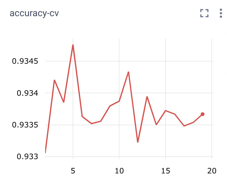
Figure 8.9 – Accuracy versus the number of folds for the k-nearest neighbor classifier

9. Now we can compare all of the produced models. Since the current Comet project does not contain only the experiments just completed, but also those executed at the beginning of this section, we need to build a filter that shows only the latest experiments. These experiments have a tag equal to kfold. We can build a filter in the Comet dashboard, as explained in Chapter 4, to select only those experiments. You can select the Filters button and then Add filter | tag | is | kfold | Done. You should be able to see only the experiments associated with a variable number of folds, as shown in the following figure:

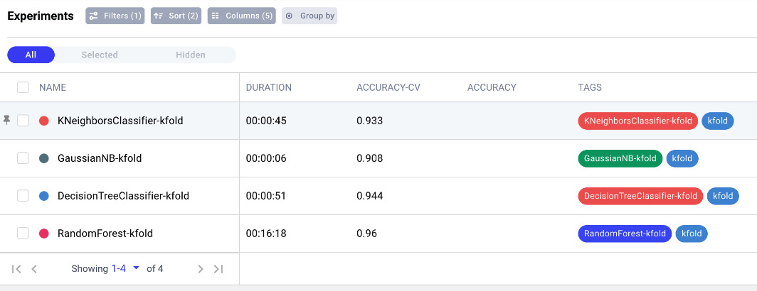
Figure 8.10 – The experiments with a tag equal to kfold shown in the Comet dashboard

10. In Comet, you can add a new panel that shows the accuracy compared to the number of folds for all the experiments. You can click on Add | New Panel | BUILT-IN | Line Chart. On the Y-axis, you can select accuracy-cv and then leave the other fields to the default values. Finally, click on Done. The following figure shows the resulting panel:

Figure 8.11 – Accuracy versus the number of folds for all of the algorithms

The panel is interactive, so if you click on a line, you should see the name of the associated model.

The implemented code returns the best number of folds for each model; thus, we can use the obtained values to perform model optimization. So, you are ready to move on to the next step: performing hyperparameters tuning with cross-validation.

Performing hyperparameters tuning with cross-validation

In Chapter 4, Workspaces, Projects, Experiments and Models, you have already learned the concept of Comet Optimizer, which permits you to perform model optimization. In this section, you will use the GridSearchCV() class provided by scikit-learn to tune the hyperparameters of each model.

We will perform the following steps:

1. We define the following function named run_experiment_grid_search():

   from sklearn.model_selection import GridSearchCV

   def run_experiment_grid_search(ModelClass, name, n_splits, params):

       model = ModelClass()

       clf = GridSearchCV(model, params, cv = n_splits)

       clf.fit(X_train, y_train)

       

       for i in range(len(clf.cv_results_['params'])):

           experiment = Experiment()

           experiment.add_tag(name + '-gs')

      experiment.add_tag('gs')

           for k,v in clf.cv_results_.items():

               if k == "params":

                   experiment.log_parameters(v[i])

               else:

                   experiment.log_metric(k,v[i])

The function receives the same parameters as the run_experiment() function as well as the dictionary of parameters to tune. Then, it builds a GridSearchCV() object with the model passed as an argument and fits it. Finally, for each tested model, the function builds a Comet Experiment and logs its parameters and its metrics.

2. We run the experiments and then we access the associated project in Comet. Since we have saved the experiments in the same project as the cross-validation example, we need to build a filter that shows only the experiments related to hyperparameter tuning. In the Comet dashboard, you can select the Filters button and then Add filter | tag | is | gs | Done.
3. Now we group experiments by model. To perform this operation, you can click on the Group by button and then Tags | Done.
4. You can select the columns to show by clicking on the columns button and adding the columns you prefer. For example, you could choose the parameters you have tuned.
5. Finally, you can sort results by decreasing the mean test score by clicking on the Sort button and then selecting the mean test score as the criterion. You can also click on the bottom arrow to set the decreasing order. You should also delete all of the other parameters appearing in the popup window by simply clicking on the X button. The following figure shows a piece of the resulting screen for the decision tree classifier:

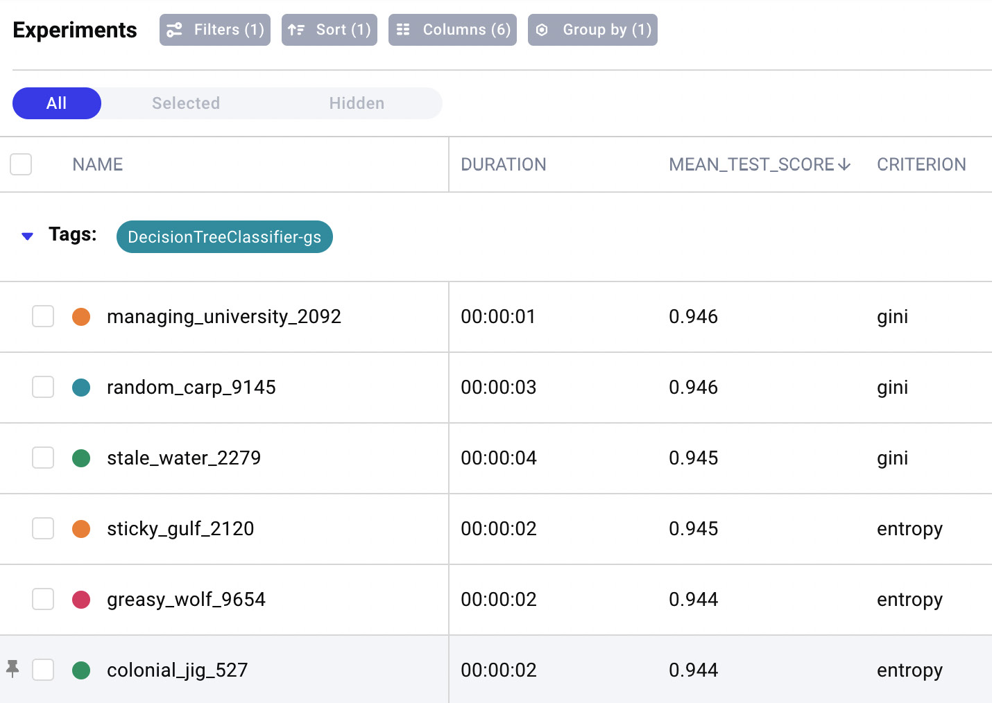
Figure 8.12 – The results of experiments in Comet for the decision tree classifier

The previous figure shows the duration, the main test score (accuracy), and the tested criterion for each experiment with the decision tree classifier. Experiments are ordered by decreasing the mean test scores, thus making it easy to recognize the best model.

6. Eventually, we can select the best model for our purpose from the different algorithms we tested. For example, we could select the best model that has a mean test score greater than 0.94 and a duration less than or equal to 1 second. You can perform this task easily in Comet as follows:
   1. You can select the Filters button, remove the current filter, and then select Add filter | mean_test_score | greater or equal | 0.9465660707805703 | Done.
   2. Then, you can add another filter remaining on the same popup window and click on Add filter | duration | less or equal | 1 sec | Done. You should see the best model, as shown in the following figure:

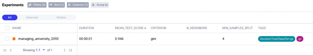
Figure 8.13 – The best model of the experiments

The best model is the decision tree with a mean test score equal to 0.946 and a duration of 1 second.

Now that you have learned how to select the best model using Comet, we can move on to the next step: calculating the SHAP value.

Calculating the SHAP value

In the Comet dashboard, you have seen that the best model is a decision tree with the following parameters:

• min_samples_split=4
• criterion='gini'

We can build a new experiment for this model and calculate the Shapley values for a single observation.

We proceed as follows:

1. First, we import all the needed libraries and build a Comet experiment as follows:

   from comet_ml import Experiment

   import shap

   shap.initjs()

   experiment = Experiment()

   experiment.set_name('BestModel')

2. Then, we build and train the model as follows:

   from sklearn.tree import DecisionTreeClassifier

   import numpy as np

   model = DecisionTreeClassifier(min_samples_split=4, criterion='gini')

   model.fit(X_train,y_train)

3. Since the model is a decision tree, we create a TreeExplainer object as follows:

   explainer = shap.TreeExplainer(model)

4. For simplicity, we decide to calculate the Shapley value related to the first sample in the test set, so we extract it as follows:

   sample = X_test.iloc[0]

5. Now we generate the decision plot. Since our model is a classifier, we should calculate the Shapley value for each target class. Thus, we define a function, which receives as input the target class (either 0 or 1), and plots the decision plot, as follows:

   def decision_plot(target):

       print(f"target: {target}")

       shap_values = explainer.shap_values(sample)[target]

       print(f"expected value: {explainer.expected_value[target]}")

       shap.decision_plot(explainer.expected_value[target], shap_values, sample)

The function calculates the Shapley values by calling the shap_values() method of the explainer. Then, it calls the decision_plot() function, which receives as input the expected value, the Shapley values, and the original sample.

6. We call the decision_plot() function for each target class as follows:

   decision_plot(0)

   decision_plot(1)

The following figure shows the resulting plots:

Figure 8.14 – The decision plot

On the left, there is the decision plot related to target class 0, while on the right we see the plot for target class 1. The vertical line represents the predicted value for each class. You can see that the predicted value for target class 0 is greater than that obtained for target class 1. This corresponds to real data in the test set where the actual class is 0. The decision plot shows the contribution of each feature (available on the left of the figure) to the final result. The red lines indicate a positive contribution, whereas the blue lines indicate a negative contribution.

7. Now, we build a summary plot as follows:

   shap_values = explainer.shap_values(X_test)

   shap.summary_plot(shap_values, X_test)

First, we extract the Shapley values from the explainer through the shap_values() method, then we call the summary_plot() function for all of the observations in the test set. The following figure shows the resulting plot:

Figure 8.15 – The summary plot

The preceding figure shows how the average Shapley value over all of the observations in the test set depends on the input features. You can see that depth is the most influential feature, followed by carat and price. The less important feature is clarity.

8. We run the experiment and we can see the results in Comet, in the Graphics section, as shown in the following figure:

Figure 8.16 – The logged Shapley graphs in Comet

The Comet experiment class has automatically logged the plots produced by shap.

Now that you have learned how to calculate the Shapley value and log it in Comet, we can move on to the final step: building the final report.

Building the final report

Now you are ready to build the final report. In this example, we will build a simple report with the graphs we just produced. As a further exercise, you could improve them by applying the concepts learned in Chapter 5, Building a Narrative in Comet. You will create a report with the following three sections:

• Cross-validation
• Hyperparameter tuning
• The Shapley value

Let’s start with the first section: cross-validation.

Cross-validation

In the Comet dashboard, you can perform the following operations:

1. Click on the Reports tab, then on New Report add a report name, such as Selecting the best model for diamond cut prediction. Finally, click on Save.
2. Come back to your main project by simply clicking on the project name on the path bar located in the top-left corner of the screen, as shown in the following figure:

Figure 8.17 – A quick way to come back to the main project through the path bar

3. In the Panels section, you should be able to see the graphs described in Figure 8.8 and Figure 8.11. If not, you can view them by removing all of the filters.
4. Click on the Add button, then Add to report, then your report name. A new section is added to your report containing the graphs. If you access the report, you can customize the section we just created.

Hyperparameter tuning

To add a new section in the report on hyperparameter tuning, you can perform the following operations:

1. You can create a new section in the report related to hyperparameter tuning. To add a new section, simply click at the end of the preceding section. A new button appears called Add section here. You can click on it to add a new section.
2. Under the Experiments part of the new section, you can select Add filter | tag | is | gs. We are simply repeating the steps performed for cross-validation in the preceding section, this time for hyperparameter tuning. If you want to add all of the experiments to the panel, you should click on the arrow near the Show 1-25 text button, located at the bottom right part of the section, and select 50.
3. Then, click on Add Panel | BUILT-IN | Bar Chart | Add. Now you can customize your graph by selecting the mean_test_score for the Y-Axis as well as selecting the Y-Axis ranges. Finally, click on the Done button.

The Shapley value

You can add a new section to the report, as described in the preceding section. Then, within this new section, you can perform the following operations:

1. Under the Experiments part of the new section, you can select Add filter | Name | is | BestModel.
2. Now you can add a panel by clicking on the Add Panel button, then FEATURED |Show images | Add | Done.
3. A new panel is added to the report containing the figures described in Figure 8.16.

The report is finally ready. You can further improve it by applying the techniques described in the previous chapters.

Summary

We just completed the journey to building a machine learning model in scikit-learn and tracking it in Comet!

Throughout this chapter, we described some general concepts regarding machine learning as well as the main structure of the scikit-learn package. We also illustrated some important concepts, such as cross-validation, hyperparameter tuning, and the Shapley value.

In the last part of the chapter, you implemented a practical use case that showed you how to track some machine learning experiments in Comet as well as how to build a report with the results of the experiments.

In the next chapter, we will review the basic concepts related to natural language processing and how to perform it in Comet.

Further reading

• Géron, A. (2019). Hands-on Machine Learning with Scikit-Learn, Keras, and TensorFlow: Concepts, Tools, and Techniques to Build Intelligent Systems. O’Reilly Media, Inc.
• Raschka, S. Liu, Y.H. and Mirjalili V. (2022). P Machine Learning with PyTorch and Scikit-Learn. Packt Publishing Ltd.