
Chapter 4: Workspaces, Projects, Experiments, and Models
Comet is an experimentation platform that permits you to track, monitor, and compare experiments within a data science project. So far, you have learned some basic concepts, including how to create and deal with workspaces, projects, experiments, panels, and reports. You have also learned how to compare experiments, customize panels, and store models in the Comet Registry.
In this chapter, you will deepen your understanding of some concepts regarding Comet, including how to add collaborators to your workspaces or projects, how to publish your projects, advanced techniques to manage experiments, and how to perform parameter optimization in Comet. In addition, you will learn how to implement a Comet experiment using R or Java as the main programming language. Finally, you will extend the basic examples implemented in Chapter 1, An Overview of Comet, with the advanced concepts learned in this chapter.
In detail, the chapter is organized as follows:
- Exploring the Comet user interface (UI)
- Using experiments and models
- Exploring other languages supported by Comet
- First use case – offline and existing experiments
- Second use case – model optimization
Before describing the advanced concepts behind Comet, let’s install all the packages needed to run the code and the experiments contained in this chapter.
Technical requirements
We will run the experiments and code in this chapter using Python, R, and Java. We'll describe the required packages for each programming language separately, starting with Python.
Python
For Python, we will use Python 3.8. You can download it from the official website at https://www.python.org/downloads/ and choose the 3.8 version.
The examples described in this chapter use the following Python packages:
- comet-ml 3.23.0
- matplotlib 3.4.3
- numpy 1.19.5
- pandas 1.3.4
- scikit-learn 1.0
We have already described the first five packages and how to install them in Chapter 1, An Overview of Comet, so please refer back to that for further details on installation.
R
R is a very popular language for statistical computing. You can use it as a valid alternative to Python since it also provides many libraries for machine learning (ML) and data science in general. You can download it from the R official website, available at this link: https://cran.rstudio.com/index.html. You should choose the version available for your operating system, and install it.
We will use the following R packages:
- caret
- cometr
- Metrics
caret (short for Classification And REgression Training) is an R package for ML. You can install it by running the following command from the R terminal:
install.packages('caret')
cometr is the official package provided by Comet to use Comet in R. You can install it by running the following command from the R terminal:
install.packages("cometr")
For more details on how to install cometr, you can refer to the Comet official documentation, available at this link: https://github.com/comet-ml/cometr.
Metrics is an R package that implements some evaluation metrics. You can install it by running the following command from the R terminal:
install.packages("Metrics")
For more details on how to install Metrics, you can refer to the Metrics official documentation, available at this link: https://cran.r-project.org/web/packages/Metrics/index.html.
Java
Java is a programming language for building applications. Although it does not support data science natively, it can also be used to implement data science projects. Many implementations of Java exist. In this chapter, we will use the Java Standard Edition (SE) Software Development Kit 17.0.2 (SDK 17), provided by Oracle. It can be used under the Oracle No-Fee Terms and Conditions (NFTC) license. You can download the Java SDK from this link: https://www.oracle.com/java/technologies/downloads/#java17. To make it work, you should follow the installation instructions available at this link: https://docs.oracle.com/en/java/javase/17/install/overview-jdk-installation.html#GUID-8677A77F-231A-40F7-98B9-1FD0B48C346A.
To facilitate the installation of the various packages used in this chapter, we also install Apache Maven, which is a tool to build, manage, and run Java applications. You can download the last release of Apache Maven from this link: https://maven.apache.org/download.cgi. To make Apache Maven work properly, please make sure that your JAVA_HOME environment variable is properly set.
We will use the following Java packages:
- comet-java-sdk-1.1.10
- weka 3.8.6
comet-java-sdk-1.1.10 is a Java package provided by Comet to interact with the Comet platform. You can download it from the Comet official repository, available at the following link: https://github.com/comet-ml/comet-java-sdk/releases. You should download the source file.
Once downloaded, you can do the following:
- Place the file wherever you like in your filesystem.
- Unzip the file.
- Enter the unzipped directory.
- Run the following command:
mvn clean install
Installation may fail, due to some dependencies on some external files in the example directory. If this is the case for you, you can edit the pom.xml file by commenting on the following line:
<module>comet-examples</module>
- Finally, you save the file and run the previous command again.
weka is a Java package for ML. To install it, you can follow the weka official documentation available at this link: https://waikato.github.io/weka-wiki/maven/. Then, proceed as follows:
- You can download the weka Java ARchive (JAR) file from Maven Central, available at this link: https://search.maven.org/search?q=a:weka-stable.
- Then, from the directory where you placed the JAR file, you can run the following command in a terminal:
mvn install:install-file
-Dfile=weka-stable-3.8.6.jar
-DgroupId= nz.ac.waikato.cms.weka:weka-stable:3.8.6
-DartifactId=weka-stable
-Dversion=3.8.6
-Dpackaging=jar
-DgeneratePom=true
This command will add the weka libraries to the Maven repository.
Now that you have set up the environment by installing all the needed packages, we can move to the next step: exploring the Comet UI—including workspaces and projects.
Exploring the Comet UI
The Comet UI provides a very useful dashboard that you can use to organize and track experiments. As already described in Chapter 1, An Overview of Comet, the Comet UI is organized into workspaces and projects. Conceptually, a workspace is a container for similar projects, while a project is a container for experiments involving the same task.
In this section, you will learn some advanced concepts regarding workspaces and projects. So, let’s start with the first one: workspaces.
Workspaces
A Comet workspace is a collection of projects. In Chapter 1, An Overview of Comet, you have already learned how to create a new workspace and how to add a new project to an existing workspace. In this section, you will learn how to add collaborators to a workspace.
To add a collaborator to a workspace, you need to sign up for at least a Teams plan or, alternatively, an Academic plan, which is free, as explained in Chapter 1, An Overview of Comet. Depending on your plan, you can add a number of of collaborators to your workspace.
To add a new collaborator, proceed as follows:
- In the Comet dashboard, you can click your username avatar in the top-right part of the screen. You should make sure that your workspace is the current workspace. If not, you can change it, by following the procedure described in Chapter 1, An Overview of Comet.
- Click Settings from the drop-down menu. Then, click Collaborators | +Collaborators. A popup should open, like the one shown in the following screenshot:

Figure 4.1 – Popup to add new collaborators
You have two options to add a new collaborator: by inviting them by email or by searching for them by username. In this last case, you can also specify their role: Admin or Member.
- Click the Invite button. The collaborator will receive a notification of the invite. When they accept it, they are ready to work with you.
Now that you have learned how to add new collaborators to a workspace, let’s move on to review some advanced concepts on projects.
Projects
A Comet project is a collection of experiments. In Chapter 1, An Overview of Comet, you have already learned how to create a new project. In this section, we will describe how to do the following:
- Set the project visibility.
- Share a project.
To set the project visibility, proceed as follows:
- Access the workspace containing the project.
- Select the gear shape button corresponding to your project, as shown in the following screenshot:

Figure 4.2 – Gear shape button corresponding to the pandas-profiles project
The button is located in the last column of the row defining your project.
- Select the Edit menu item.
- Choose the project visibility and click on Update. You can choose either Private or Public. If you choose to make your project public, the project will be available at this link: https://www.comet.ml/<WORKSPACE NAME>/<PROJECT NAME>/view.
As with workspaces, you can decide to share a single project with a collaborator. Again, you need at least a Teams or an Academic plan.
To share a project with a collaborator, proceed as follows:
- From the project's main dashboard, select the Manage tab.
- If you want to share your project with your collaborators in read-only mode, you can click Create Sharable Link. In this case, they will be able only to read the project; they will not be able to edit it.
- Alternatively, you can click the +Collaborators button to share the project with one or more collaborators, who will also be able to edit your project. The procedure is similar to that described for workspaces.
Now that you have learned some advanced concepts on projects and workspaces, we can move on to investigate some other aspects of experiments and models.
Using experiments and models
Experiments and models are the core of a Comet project because they permit you to track and monitor all your data science projects. You have already learned the basic concepts behind experiments and models in Chapter 1, An Overview of Comet, and Chapter 3, Model Evaluation in Comet. In this section, you will learn some advanced topics involving offline and existing experiments, as well as model optimization.
This section is organized as follows:
- Experiments
- Models
Let’s start from the first point: experiments.
Experiments
A Comet experiment is a process that permits you to track your variables while the underlying conditions change. You have already learned the basic concepts behind Comet experiments in Chapter 1, An Overview of Comet. You have already seen the Experiment class, which permits you to connect directly with Comet through an available internet connection. However, it may happen that at a certain time your internet connection is not available for some reason, or you need to stop your experiments and then continue them after a given period of time. To deal with these situations, Comet provides three additional experiment classes, as outlined here:
- Offline experiment—If you do not have an internet connection, you can create an OfflineExperiment() object, which permits you to store your experiment locally on your filesystem. Then, you can upload the experiment to Comet in a second instance. You can create an offline experiment like this:
from comet_ml import OfflineExperiment
experiment = OfflineExperiment(offline_directory="PATH/TO/THE/OUTPUT/DIRECTORY")
The offline_directory parameter specifies the output directory where the experiment will be saved. Once you have created an experiment, you can use it as you usually do with the standard Experiment class. When the experiment ends, the output directory will contain a zipped file. You can upload it by running it through the command-line utility, like so:
comet upload PATH/TO/THE/ZIP/FILE
- Existing experiment—You can continue an existing experiment by creating an ExistingExperiment() object, which receives as input the key of the experiment to continue. This is particularly useful when you want to separate the training and test phases of an experiment, or if you want to improve a previous experiment. You can create an existing experiment like this:
from comet_ml import ExistingExperiment
experiment = ExistingExperiment(previous_experiment= "EXPERIMENT_KEY ")
To use the ExistingExperiment() object, you need to know the experiment key in advance, which you can specify through the previous_experiment input parameter.
- Offline existing experiment—You can continue an existing experiment offline. This is a combination of the previous two cases. In this case, you should create an ExistingOfflineExperiment() object, as specified in the following piece of code:
from comet_ml import ExistingOfflineExperiment
experiment = ExistingOfflineExperiment(offline_directory= "PATH/TO/THE/OUTPUT/DIRECTORY", previous_experiment= "EXPERIMENT_KEY ")
You must specify both the offline_directory parameter and the experiment key. If you want to upload an experiment in Comet, you should run the following command from a terminal:
comet upload PATH/TO/THE/ZIP/FILE
You will practice with the different types of experiments at the end of this chapter, when we will extend the first use case described in Chapter 1, An Overview of Comet.
Now that you have learned some advanced concepts regarding experiments, we can move to the next point: models.
Models
A Comet model is an algorithm that learns a pattern from known data and uses it to make predictions on unknown data. You can build your model for different purposes, including data classification, regression, natural language processing (NLP), time-series forecasting, and so on.
You have already learned how to track and organize models in Comet in Chapter 3, Model Evaluation in Comet. Comet also provides an additional feature that permits you to optimize your models. This feature is called an Optimizer. In this section, we will describe how to build an Optimizer in Comet, while in Chapter 8, Comet for Machine Learning, Chapter 9, Comet for Natural Language Processing, Chapter 10, Comet for Deep Learning, and Chapter 11, Comet for Time Series Analysis, you will review the main techniques for model optimization.
You can use a Comet Optimizer for tuning the hyperparameters of your model, by choosing one of the supported optimization algorithms: Grid, Random, and Bayes. If you want to learn more details about the optimization algorithms, you can refer to the Comet official documentation, available at the following link: https://www.comet.ml/docs/python-sdk/introduction-optimizer/#optimizer-algorithms.
Follow these next steps:
- You can create a Comet Optimizer like this:
from comet_ml import Optimizer
optimizer = Optimizer(config)
We create an Optimizer object, which receives as input some configuration parameters that include the metric to maximize/minimize, the number of trials, the optimization algorithm, and the parameters to test.
- You can define the configuration parameters like so:
config = {"algorithm": <MY_OPTIMIZATION_ALGORITHM>,
"spec": {
"objective": <MINIMIZE/MAXIMIZE>,
"metric": <METRIC>,
},
"trials": <NUMBER OF TRIALS>,
"parameters": [LIST OF PARAMETERS],
"name": <OPTMIZER NAME>
}
The config object is a dictionary that includes all configuration parameters. In addition to the parameters listed in the previous piece of code, you can define other parameters, as specified in the Comet official documentation.
- The list of parameters includes all specific parameters to test, and for each of them, you must specify a range of possible values (integer, categorical, and so on). Depending on the type of parameter, the syntax changes. For an integer type, you should specify the minimum and maximum values, as well as the scaling type, as shown in the following piece of code:
{<PARAMETER-NAME>:
{"type": "integer",
"scalingType": "linear" | "uniform" | "normal" | "loguniform" | "lognormal",
"min": <MIN-VALUE>,
"max": <MAX-VALUE>,
}
The PARAMETER-NAME value depends on the specific algorithm. For example, for a K-Nearest Neighbors (KNN) classifier, you may need to hypertune the number of neighbors.
- If you want to hypertune a categorical parameter, you can use the following syntax:
{<PARAMETER-NAME>:
{"type": "categorical",
"values": ["LIST", "OF", "CATEGORIES"]
}
}
The "values" key contains a list of all possible categories to test.
When you create an Optimizer object, the system will create an experiment for each combination of parameters included in the configuration. You can access a list of experiments by executing the following code:
optimizer.get_experiments():
By iterating over the list of experiments, you can access every single parameter, and use it to fit a different model, as follows:
for experiment in opt.get_experiments():
param1 = experiment.get_parameter("param1")
# create, fit and test the model with param 1
The previous code shows how to retrieve each parameter, which you can use as you want to create, fit, and test your preferred model. The commented line indicates that the code you should write after retrieving a parameter depends on the model you want to implement.
Once you have run all the experiments, you will see the results in Comet. You will implement a practical use case at the end of this chapter, in the Second use case – model optimization section.
Now that you have learned some advanced concepts regarding experiments and models, we can move to the next step: other languages supported by Comet.
Exploring other languages supported by Comet
So far, you have learned how to use Comet in Python. However, Comet also supports other programming languages. The concepts learned so far on experiments, panels, and so on are also valid with the other languages supported by Comet.
In this section, you will apply the concepts already acquired in the previous chapters to the R and Java languages. So, if you are not interested in programming in these languages, you can skip this section and go directly to the next one, First use case – offline and existing experiments.
In this section, you will learn how to build and run an experiment in the following languages:
- R
- Java
Let’s start with the first language: R.
R
Let’s suppose that you have already created a new project in Comet and obtained an application programming interface (API) key, as described in Chapter 1, An Overview of Comet. As described in that chapter, you should define a configuration file named .comet.yml that should contain all configuration parameters, as shown in the following piece of code:
COMET_WORKSPACE: MY_WORKSPACE
COMET_PROJECT_NAME: MY_PROJECT_NAME
COMET_API_KEY: MY_API_KEY
The configuration file should contain the workspace name, the project name, and the API key. You should save the file either in the working directory or in your home directory.
In this section, you will use the caret package to perform an ML task in R. The section is divided into the following parts:
- Exploring the cometr package
- Reviewing the caret package
- Running a practical example
Let’s start with the first part: exploring the cometr package.
Exploring the cometr package
The cometr package provides functions to interact with the Comet platform. For a list of available functions, you can refer to the Comet official documentation, available at this link: https://www.comet.ml/docs/r-sdk/getting-started/. Here is a list of the most common functions:
- create_experiment()/create_project()—To create a new experiment/project
- get_experiments()/get_projects()/get_workspaces()—To get a list of experiments/projects/workspaces
You can use the create_experiment() function to create an experiment() object. Once you have created an experiment() object, you can log parameters, metrics, and objects, as you usually do in Python. For a list of available methods, you can refer to the Comet official documentation, available at this link: https://www.comet.ml/docs/r-sdk/Experiment/. Here is a list of the most common methods available for the experiment() object:
- log_metric()/log_parameter()/log_html()/log_code()/log_graph()/log_other()—To log a metric, a parameter, a HyperText Markup Language (HTML) page, code, a graph, or other objects
- upload_asset()—To upload an asset to the Comet platform
Now that you have learned the basic functions and methods provided by the cometr package, we can briefly review the caret package.
Reviewing the caret package
The caret package provides the following main features to perform ML in R:
- Preprocessing, which permits you to clean, normalize, and center your dataset, as well as performing other preprocessing operations. To perform preprocessing, you can use the preProcess() function, as follows:
X_preprocessed <- preProcess(X, method = c("center", "scale"))
The function takes a dataset as input, as well as a list of operations to perform. In the example, we performed centering and scaling.
- Data splitting, which permits you to split your data into training and test sets. You can use the createPartition() function to split a dataset into training and test sets, as illustrated in the following piece of code:
index <- createDataPartition(dataset, p = .8,
list = FALSE,
times = 1)
The p parameter specifies the training set size in terms of probability. Setting the list = FALSE parameter avoids returning the data as a list, and the times parameter sets the number of splits to return. The function returns a list of indices belonging to the first partition. So, you need to create two variables—one for the training set and the other for the test set containing the selected indices, as follows:
training <- df[index,]
test <- df[-index,]
df is the original dataset loaded as a DataFrame.
- Model training permits you to train a specific model. The caret package provides the train() method to train a model, as shown in the following piece of code:
model <- train(class ~ ., method='knn', data = training, metric='Accuracy')
The first argument is the predictor, which permits you to select the output. You can also specify the type of model through the method argument, the input data, and the metric to calculate. You can even set a training control for hyperparameter tuning. For more details on this aspect, you can refer to the caret official documentation, available at the following link: https://topepo.github.io/caret/model-training-and-tuning.html#model-training-and-parameter-tuning.
- Model prediction, which permits you to predict the output for new unseen data. You can use the predict() function like so:
y_pred <- predict(model, X_test)
- Model evaluation, which permits you to evaluate the performance of the model. Depending on the specific task, you can calculate different metrics. For more details, you can refer to the caret official documentation, available at the following link: https://topepo.github.io/caret/measuring-performance.html. Since the caret package does not provide a direct method to calculate the accuracy, in the example described in the next section, we will use the Metrics package to calculate it.
Now that you have learned the basic concepts to build a model in caret, you can implement a practical use case.
Running a practical example
We will use the Mushrooms Classification dataset, available on Kaggle (https://www.kaggle.com/uciml/mushroom-classification) under the Creative Commons Zero (CC0) public license. Our objective is to build a classification model that predicts whether a mushroom is edible or poisonous. (You can find the full code of this example in the GitHub repository of the book, available at the following link: https://github.com/PacktPublishing/Comet-for-Data-Science/tree/main/04/r-example.)
Here are the steps we’ll take:
- Firstly, we import all the needed libraries, as follows:
library(cometr)
library(caret)
library(Metrics)
- Then, we load the dataset as a DataFrame, like this:
df <- read.csv('mushrooms.csv')
The dataset contains 8,124 rows and 23 columns. The following screenshot shows the first 10 rows of the dataset:

Figure 4.3 – An extract of the mushrooms dataset
- The first column of the dataset contains the target class. We can also note that all columns of the dataset contain categorical variables. Thus, we convert them into numerical values, as shown in the following piece of code:
for(i in 2:ncol(df)) {
df[ , i] <- as.numeric(factor(df[ , i], levels = unique(df[ , i]), exclude = NULL))
}
In the for loop, we start from the second column, because the first one is the target class.
- Now, we encode the target class, as follows:
df$class <- as.factor(df$class)
With respect to the previous code, we do not convert the class to numeric values.
- We create a Comet experiment by executing the following code:
experiment <- create_experiment()
- Now, we are ready to create a model. The idea is to split the dataset into batches, and track the performance of the model for each step. We use a KNN classifier to perform the classification task. The following code snippet shows how we train and test the model, as well as how we log all metrics in Comet:
set.seed(10)
n <- dim(df)[1]
burst <- 1000
for (i in seq(200, n+burst, by=burst)) {
if(i > n)
i = n
dft <- df[c(1:i),]
index <- createDataPartition(y = dft$class, times = 1, p = 0.7, list = FALSE)
training <- dft[index,]
test <- dft[-index,]
model <- train(class ~ ., method='knn', data = training, metric='Accuracy')
test$pred <- predict(model, test)
acc <- accuracy(test$class, test$pred)
test$factor_pred <- as.factor(test$pred)
test$factor_truth <- as.factor(test$class)
precision <- posPredValue(test$factor_truth, test$factor_pred)
recall <- sensitivity(test$factor_truth, test$factor_pred)
F1 <- (2 * precision * recall) / (precision + recall)
experiment$log_metric("accuracy", acc, step=i)
experiment$log_metric("precision", precision, step=i)
experiment$log_metric("recall", recall, step=i)
experiment$log_metric("F1", F1, step=i)
}
Firstly, we set the seed to 10 to make the experiment reproducible. For each batch, we split the dataset into training and test through the createDataPartition() function, provided by the caret library. Then, we train the model, through the train() function. We also specify that we want to optimize the accuracy. Now, we test the model performance through the predict() function, and we calculate the accuracy, the precision, the recall, and the F1-score. Finally, we log all the calculated metrics in Comet, through the log_metric() method of the experiment class.
- Finally, we terminate the experiment, as follows:
experiment$stop()
- We run the code from the R console, as follows:
setwd('/PATH/TO/THE/DIRECTORY/CONTAINING/YOUR/CODE')
source('script.R')
Firstly, we need to change directory through the setwd() function, then we run the code, through the source() function.
- Now, the experiment is available in Comet, as shown in the following screenshot:
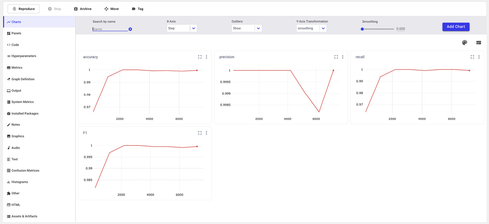
Figure 4.4 – Output of the experiment in Comet
Figure 4.4 shows the output of the experiment in Comet, with a focus on the accuracy, precision, recall, and F1-score curves.
Now that you have learned how to build a Comet experiment in R, we can move on to the next step: building a Comet experiment in Java.
Java
Let’s suppose that you have already created a new project in Comet and you already have an API key, as described in Chapter 1, An Overview of Comet. Let’s further suppose that you have already created a Maven project with a pom.xml file Take the following steps:.
- You should add the Comet library to the dependency section of your pom.xml file, as follows:
<dependency>
<groupId>ml.comet</groupId>
<artifactId>comet-java-client</artifactId>
<version>1.1.10</version>
</dependency>
In the previous code snippet, we have added comet-java-client version 1.1.10 to our project.
- You should also configure a file named application.conf, as follows:
comet {
baseUrl = "https://www.comet.ml"
apiKey = "YOUR API KEY"
project = "YOUR PROJECT NAME"
workspace = "YOUR EXPERIMENT"
}
The file contains configuration parameters to access the Comet platform.
- You should add the application.conf file to the project classpath in the pom.xml file, as follows:
<resources>
<resource>
<directory>PATH/TO/THE/CONF/FILE</directory>
</resource>
</resources>
In this section, you will use the weka package to perform an ML task in Java. The section is divided into the following parts:
- Exploring the ml.comet package
- Reviewing the weka package
- Running a practical example
Let’s start from the first part: exploring the ml.comet package.
Exploring the ml.comet package
The ml.comet package provides functions to interact with the Comet platform. For a list of available classes and functions, you can refer to the Comet official documentation, available at this link: https://www.comet.ml/docs/java-sdk/getting-started/. Comet provides the OnlineExperimentBuilder class to create experiments, and the OnlineExperiment interface to manage experiments. You can create a new experiment by running the following code:
import ml.comet.experiment.ExperimentBuilder;
import ml.comet.experiment.OnlineExperiment;
OnlineExperiment experiment = ExperimentBuilder.OnlineExperiment().build();
The previous code creates a new experiment() object you can use to log and track your experiments.
Similar to the experiment class defined for the other programming languages, the OnlineExperiment interface also provides the following methods:
- logMetric()/logModel()/logArtifact()/logParameter()—To log a metric, a model, an artifact or a parameter
- setEpoch()/setStep()—To set the current epoch/step of the experiment
- nextEpoch()/nextStep()—To increment the current epoch/step of the experiment
The previous list of methods contains the most important methods provided by the OnlineExperiment interface. You can refer to the Comet official documentation for a complete list of methods.
Now that you have learned the basic functions and methods provided by the ml.comet package, we can briefly review the weka package.
Reviewing the weka package
The weka package contains many subpackages to perform ML tasks. Among them, we will use the following ones:
- core, which contains the main classes and functions to prepare data for further analysis. In particular, you can load a comma-separated values (CSV) file, as follows:
CSVLoader loader = new CSVLoader();
loader.setSource(new File("/path/to/csv/file.csv"));
Instances dataset = loader.getDataSet();
- classifiers, which contains all algorithms used to perform supervised learning (SL). Algorithms related to regression are available under the classifiers.functions subpackage. To build a classifier and train it, you can run the following code:
MyModel model = new MyModel();
model.buildClassifier(training);
The MyModel() class is one of the classes provided by the classifiers subpackage, such as IBk() to implement a KNN classifier. The classifiers package also contains a class named Evaluation that you can use to perform model evaluation. You will see a practical example of how to use it in the next section.
Now that you have reviewed the basic packages provided by the weka package, we can move to the next step: implementing a practical use case.
Running a practical example
We will use the Mushrooms Classification dataset, available on Kaggle (https://www.kaggle.com/uciml/mushroom-classification) under the CC0 public license. We have already used it in the previous section. We will implement the same use case as the previous section—that is, build a classification model that predicts whether a mushroom is edible or poisonous. We will use the weka package to perform ML tasks.
(You can find the full code of this example in the GitHub repository of the book, available at the following link: https://github.com/PacktPublishing/Comet-for-Data-Science/tree/main/04/java-example.)
Here are the steps we’ll take:
- Firstly, we create a new Java script named KNN.java and we set the package name, as follows:
package packt.comet;
- Then, we import all the needed classes, like so:
import ml.comet.experiment.ExperimentBuilder;
import ml.comet.experiment.OnlineExperiment;
import weka.core.Instances;
import weka.core.converters.CSVLoader;
import weka.classifiers.Classifier;
import weka.classifiers.lazy.IBk;
import weka.classifiers.Evaluation;
import java.util.Random;
import java.io.File;
From ml.comet, we have imported the classes needed to interact with Comet; from weka, we have imported the classes needed to load the CSV file and to perform classification, and from java, we have imported some utility functions.
- Now, we define a class named KNN that will contain the code, as follows:
public class KNN {
public static void main( String[] args )
{...}
}
We have also defined a main() method, which will contain all the following code.
- Within the main() method, we create a new experiment, as follows:
OnlineExperiment experiment = ExperimentBuilder.OnlineExperiment().build();
experiment.setExperimentName("KNN");
We also set the experiment name through the setExperimentName() method.
- We load the file as an Instances object, as follows:
try {
CSVLoader loader = new CSVLoader();
loader.setSource(new
File("src/main/resources/mushrooms.csv"));
Instances data = loader.getDataSet();
data.setClassIndex(0);
} catch (Exception ex) {
System.err.println("Exception occurred! " + ex);
}
We also set the target class to the first column, through the setClassIndex() method provided by the Instances class.
- Now, we are ready to create a model. Similar to the previous section, we split the dataset into batches, and for each batch, we calculate the performance of the model. We use a KNN classifier to perform the classification task. The following code shows how we train and test the model, as well as how we log all metrics in Comet:
int n = data.numInstances();
for (int i = 200; i < n+1000; i+=1000) {
if(i > n) i = n;
Instances current_data = new Instances(data, 0, i);
// train test splitting
int seed = 10;
current_data.randomize(new Random(seed));
int trainSize = (int) Math.round(current_data.numInstances() * 0.7);
int testSize = current_data.numInstances() - trainSize;
Instances train = new Instances(current_data, 0, trainSize);
Instances test = new Instances(current_data, trainSize, testSize);
// train the model
IBk model = new IBk();
model.buildClassifier(train);
// evaluate the model
Evaluation eval = new Evaluation(test);
eval.evaluateModel(model,test);
double accuracy = eval.pctCorrect()/100;
experiment.logMetric("accuracy", accuracy);
experiment.setStep(i);
}
We use the IBk class provided by weka to create a KNN classifier, and the Evaluation class to evaluate the model.
- Finally, we terminate the experiment, as follows:
experiment.end();
- From the project root directory, we run the code, as follows:
mvn clean compile exec:java -Dexec.mainClass="packt.comet.KNN"
In the previous code, firstly we compile the project, and then we run it.
- We can access the results of the experiment directly in Comet, as shown in the following screenshot:

Figure 4.5 – The Comet dashboard after running the Java experiment
Figure 4.5 shows the Comet main dashboard with an accuracy graph related to the KNN experiment.
Now that you have learned some advanced concepts on Comet, you can practice with them through two practical use cases. Let’s start with the first use case: offline and existing experiments.
First use case – offline and existing experiments
In Chapter 1, An Overview of Comet, you built a simple use case that permitted you to track images in Comet. The example used 52 time series indicators related to gross domestic product (GDP) in Italy, built 52 images, and uploaded them to Comet.
During the experiment, you will surely have noticed that the loading of the images in Comet was quite slow, depending on the bandwidth available in your internet connection. In this example, you will see how to use the concepts of offline and existing experiments to make the loading process smoother. You will also see how an existing experiment can be improved at a later time.
In this example, we suppose that the code implemented in Chapter 1, An Overview of Comet, for the first use case is running. Thus, please refer to it for further details.
The full code of this example is available in the GitHub repository, at the following link: https://github.com/PacktPublishing/Comet-for-Data-Science/tree/main/04/first-use-case-advanced.
In detail, the example is organized as follows:
- Running an offline experiment
- Continuing an existing experiment
- Improving an existing experiment offline
Let’s start from the first phase: running an offline experiment.
Running an offline experiment
The idea here is to transform the online experiment described in Chapter 1, An Overview of Comet, into an offline experiment. This will permit you to upload the images in Comet in the background, once the experiment is completed.
To perform this operation, you can just change the following line of code:
from comet_ml import Experiment
experiment = Experiment()
Your code should now look like this:
from comet_ml import OfflineExperiment
experiment = OfflineExperiment(offline_directory="output")
Obviously, you need to create a directory named output in your current working directory. After running the experiment, your output directory will contain a file similar to the one shown in the following screenshot:
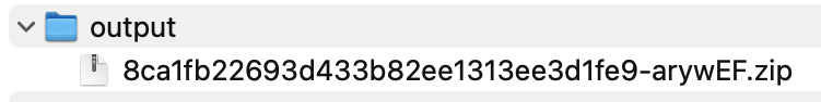
Figure 4.6 – Directory containing the offline experiment
Now, you can upload the offline experiment to Comet, as explained in the Using experiments and models section of this chapter. You should also remember to configure the .comet.config file to make the experiment work, as explained in Chapter 1, An Overview of Comet.
Now that you have built an offline experiment, we can move to the next step: continuing an existing experiment.
Continuing an existing experiment
Dividing the experiment into two parts could be an alternative to the previous strategy to save internet bandwidth. Thus, we could build an experiment that uploads to Comet the first N images, and then continue it and upload to Comet the remaining images.
Here’s how we’ll go about this:
- Firstly, we wrap the existing code to build graphs into a single function, like so:
def run_experiment(df, experiment, indicators = df.columns):
for indicator in indicators:
ts = df[indicator]
ts.dropna(inplace=True)
ts.index = ts.index.astype(int)
fig = plot_indicator(ts,indicator)
experiment.log_image(fig,name=indicator, image_format='png')
The run_experiment() function receives the df DataFrame, the experiment, and a list of indicators as input, and for each indicator, it builds and logs the corresponding plot.
- Now, you build an experiment as you usually do, as illustrated here:
from comet_ml import Experiment, ExistingExperiment
experiment = Experiment()
experiment.set_name('Track Indicators - first part')
I also set the name of the experiment through the set_name() function.
- Then, you run the experiment by tracking the first 10 experiments, as follows:
N = 10
run_experiment(df,experiment, indicators=df.columns[0:N])
- You retrieve the experiment key to continue the experiment later, as illustrated in the following code snippet:
experiment_key = experiment.get_key()
If you access the experiment in Comet, you can see an experiment called Track Indicators – first part, and, under the Graphics menu item, you will see the first 10 graphs. You will note that the uploading process was quite fast.
- Now, you can continue the previous experiment by defining an ExistingExperiment() object, as follows:
from comet_ml import ExistingExperiment
experiment = ExistingExperiment(previous_experiment=experiment_key)
experiment.set_name('Track Indicators - final')
You have also changed the name of the experiment, to track changes in the Comet dashboard.
- Now, you can run the experiment with the remaining indicators, as follows:
run_experiment(df,experiment, columns=df.columns[N:])
If you now access the Comet dashboard, you can see the experiment with a different name, Track Indicators – final, and under the Graphics section, you will see all the graphs.
Now that you have learned how to continue an existing experiment, we can move to the next step: improving an existing experiment offline.
Improving an existing experiment offline
Let’s suppose that for each indicator, you want to also plot a trendline that shows whetherthe indicator has an increasing or decreasing trend. In practice, for each indicator, you should calculate a linear regression model and then plot the resulting line. Since this operation could be time-consuming, you could decide to perform it offline and then upload the results in Comet in the background. Let’s also suppose that you know the experiment key associated with your experiment.
Here are the steps we’ll take:
- Firstly, we create an ExistingOfflineExperiment() object, as follows:
from comet_ml import ExistingOfflineExperiment
experiment = ExistingOfflineExperiment(offline_directory="output",previous_experiment=experiment_key)
We have specified the offline directory and the experiment key.
- Then, we modify the plot_indicator() function defined in Chapter 1, An Overview of Comet, to also plot the trendline, as follows:
def plot_indicator(ts, indicator,trendline):
fig_name = 'images/' + indicator.replace('/', "") + '.png'
xmin = np.min(ts.index)
xmax = np.max(ts.index)
plt.figure(figsize=(15,6))
plt.plot(ts)
plt.plot(ts.index,trendline)
plt.title(indicator)
plt.grid()
plt.savefig(fig_name)
return fig_name
- Afterward, for each indicator, we implement a linear regression model, and we plot the time series and the output of prediction through the plot_indicator() function previously defined. The code is illustrated in the following snippet:
from sklearn.linear_model import LinearRegression
for indicator in df.columns:
ts = df[indicator]
ts.dropna(inplace=True)
ts.index = ts.index.astype(int)
X = ts.index.factorize()[0].reshape(-1,1)
y = ts.values
model = LinearRegression()
model.fit(X,y)
y_pred = model.predict(X)
fig = plot_indicator(ts,indicator,y_pred)
experiment.log_image(fig,name=indicator, image_format='png', overwrite = True)
Note that we have use the LinearRegression() class provided by scikit-learn to implement the linear regression model. For each indicator, we build a graph similar to the one shown in the following screenshot:

Figure 4.7 – Graph produced for the “Agriculture, forestry, and fishing, value added” indicator
Figure 4.7 shows the trendline in orange and the indicator line in blue.
- Finally, once the experiment is completed, we upload it to Comet, like so:
comet upload PATH/TO/THE/ZIP/FILE
If you access the Comet dashboard, corresponding to your experiment, under the Graphics menu item, you will see all updated graphs, as shown in the following screenshot:
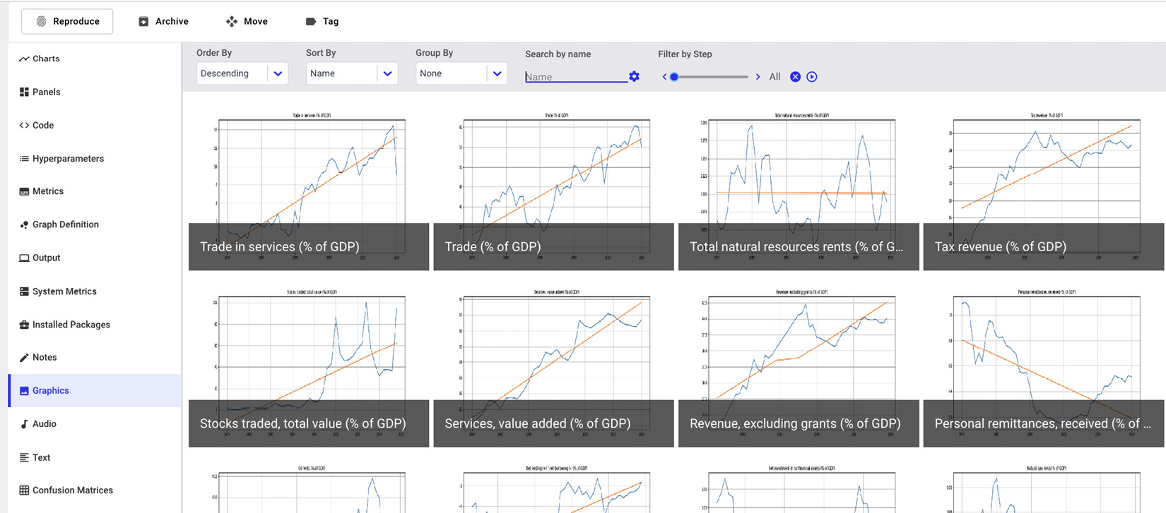
Figure 4.8 – Updated graphs under the Graphics menu item
Now that you have completed the first use case, we can move on to the second use case.
Second use case – model optimization
In Chapter 1, An Overview of Comet, you built a simple use case that permitted you to define a simple regression model and show the results in Comet. The example used the diabetes dataset provided by the scikit-learn library and calculated the mean squared error (MSE) for different values of seeds.
During the experiment, you will surely have noticed that the average MSE was about 3,000. In this example, we show how to use the concept of Optimizer to reduce the MSE value. Since the linear regression model does not provide any parameters to optimize, in this example, we will build a gradient boosting regressor model, and we will tune some of the parameters it provides.
In this example, we suppose that the code implemented in Chapter 1, An Overview of Comet, for the second use case is running. Thus, please refer to it for further details.
The full code of this example is available in the GitHub repository, at the following link: https://github.com/PacktPublishing/Comet-for-Data-Science/tree/main/04/second-use-case-advanced.
In detail, the example is organized like this:
- Creating and configuring an Optimizer
- Optimizing the model
- Showing the results in Comet
Let’s start from the first phase: creating and configuring an Optimizer.
Creating and configuring an Optimizer
We will optimize the gradient boosting regressor model by hypertuning the following parameters:
- n_estimators—The number of trees in the forest. We will test values from 100 to 110.
- max_depth—The number of leaves in each tree. We will test values from 4 to 6.
- loss—The loss function to optimize. We will test two types of loss functions: squared_error and absolute_error.
To configure the Comet Optimizer, we perform the following steps:
- We define a list of parameters, as follows:
params = {
'n_estimators':{
"type" : "integer",
"scalingType" : "linear",
"min" : 100,
"max" : 110
},
'max_depth':{
"type" : "integer",
"scalingType" : "linear",
"min" : 4,
"max" : 6
},
'loss': {
"type" : "categorical",
"values" : ['squared_error', 'absolute_error']
}
}
For each parameter, we specify the type and other properties that depend on the type of parameter (categorical or integer).
- We define a configuration variable that will be given as input to the Comet Optimizer class, as follows:
config = {
"algorithm": "grid",
"spec": {
"maxCombo": 0,
"objective": "minimize",
"metric": "loss",
"minSampleSize": 100,
"retryLimit": 20,
"retryAssignLimit": 0,
},
"trials": 1,
"parameters": params,
"name": "GB Optiimizer"
}
We choose grid as the optimization algorithm, and we specify that we want to minimize the loss function. We also set the parameters key to the params variable previously defined.
- We build the Comet Optimizer, as follows:
from comet_ml import Optimizer
opt = Optimizer(config)
We pass as the input parameter to the Optimizer class the config variable previously defined.
Now that we have set up the Comet Optimizer, we are ready to optimize the model.
Optimizing the model
Let’s suppose that you already have loaded the diabetes dataset, as described in Chapter 1, An Overview of Comet. Now, we'll build an experiment for each combination of parameters returned by the Optimizer. For each experiment, we will calculate the MSE for different values of seed, as already performed in Chapter 1, An Overview of Comet.
Here are the steps we’ll take:
- For each experiment contained in the list of experiments returned by the Comet Optimizer through the get_experiments() method, we build a GradientBoostingRegressor() object, initialized with the parameters defined for the current experiment.
- Then, for each seed instance in the list of seeds, we split the dataset into training and test sets, and we fit the current model.
- Finally, we calculate the MSE and log it in Comet through the log_metric() method.
The following code implements the previously described steps:
for experiment in opt.get_experiments():
model = GradientBoostingRegressor(
n_estimators=experiment.get_parameter("n_estimators"), max_depth=experiment.get_parameter("max_depth"), loss=experiment.get_parameter("loss"),)
for seed in seed_list:
X_train, X_test, y_train, y_test = train_test_split(X, y, test_size=0.20, random_state=seed)
model.fit(X_train, y_train)
y_pred = model.predict(X_test)
mse = mean_squared_error(y_test,y_pred)
experiment.log_metric("MSE", mse, step=seed)After running the previous code, you are ready to see the results in Comet. So, let’s move to the final step: showing the results in Comet.
Showing the results in Comet
In total, we performed 40 experiments. We can order the experiments by increasing MSE, as described in Chapter 3, Model Evaluation in Comet. The result is shown in the following screenshot:

Figure 4.9 – The Comet dashboard after ordering the experiments by increasing MSE
mushy_amberjack_2424 is the experiment with the lowest MSE. If we click on this experiment, we can view its parameters under the Hyperparameters section, as shown in the following screenshot:

Figure 4.10 – Hyperparameters menu item in the Comet dashboard
Figure 4.10 shows only a subset of the parameters.
Optionally we could log all the models, save them in the Registry, and then choose the best model to send to production, as described in Chapter 3, Model Evaluation in Comet.
This example also plots the MSE metric versus the seed, as shown in the following screenshot:

Figure 4.11 – MSE metric for the different experiments
Comet produced the previous output automatically during the running process.
Summary
We just completed the journey through advanced concepts in Comet!
Throughout this chapter, you learned how to share projects and workspaces with your collaborators, as well as how to make them public or private. In addition, you learned some advanced concepts on experiments and models.
Regarding experiments, you learned about the concept of offline experiments, which permitted you to run an experiment if the internet connection is not available. In addition, you learned about the concept of existing experiments, which permitted you to continue an experiment—for example, by enriching or extending it.
Regarding models, you learned how to optimize model parameters, through the concept of the Comet Optimizer. Using the Comet Optimizer makes it simple to choose the best parameters for a given model.
Finally, you extended the basic examples defined in Chapter 1, An Overview of Comet, with the concepts described in this chapter.
In the next chapter, you will review some concepts about data narrative and how to perform it in Comet.
Further reading
- Bhatia, A. & Kaluza, B. (2018). Machine Learning in Java: Helpful techniques to design, build, and deploy powerful machine learning applications in Java. Packt Publishing Ltd.
- Lantz, B. (2019). Machine Learning With R: Expert Techniques For Predictive Modeling. Packt Publishing Ltd.