
9
Optimizing Cloud-Native Environments
Compute, networking, and storage form the bulk of Amazon Web Services (AWS) cost and usage. We’ve covered the services that are most common in these categories, such as Amazon Elastic Compute Cloud (EC2), Amazon Simple Storage Service (S3), AWS’s various database services, and Amazon Virtual Private Cloud (VPC). However, given that AWS’ complete portfolio exceeds 200 services, we’ve only scratched the surface.
This chapter covers optimization opportunities that result from the induced demand of cloud-native environments; what I mean by this is the demand for AWS services that are more easily obtained in the cloud than from on-premises systems. For example, automatically horizontally scaling a fleet of servers is more easily done in the cloud than on-premises because if you were to horizontally scale your on-premises servers, you would first need to buy the maximum number of servers to meet your peak capacity, whereas, in a cloud environment, you simply scale when you need to and expect the cloud provider to supply your demand for servers. Also, for an on-premises machine learning (ML) workload, you need to purchase and maintain the maximum number of servers to run distributed training jobs, but in the cloud, you simply utilize the distributed training cluster through an application programming interface (API) call and once training is complete, you stop paying for (expensive) servers for ML training. We define cloud-native environments in this way and use this chapter to identify ways to optimize costs.
Although it would require more than one chapter to cover every service, we’ll look at a few and generalize optimization best practices from what we’ve seen thus far. We start with AWS Auto Scaling, which covers not only EC2 instances but containers and databases as well. Then, we’ll see the role optimization plays in an end-to-end (E2E) analytics workflow including ML. Finally, we’ll glance at a few more services and generalize based on these patterns.
In this chapter, we’re going to cover the following main topics:
- Maximizing efficiency with AWS Auto Scaling
- Optimizing analytics
- Optimizing ML
Technical requirements
To complete the exercises in this chapter, the requirements are the same as what we’ve been using in the previous chapters.
Maximizing efficiency with AWS Auto Scaling
We’ll begin by understanding auto scaling, which is the embodiment of elasticity in the cloud. After we define auto scaling, we’ll learn how you can leverage different auto-scaling policies and strategies to meet your workload requirements. Implementing auto scaling will be key in your cloud waste reduction efforts because it’s the closest thing to not paying for resources you don’t need. Let’s define what it is by looking at a simple example.
What is auto scaling?
Large social gatherings such as weddings, banquets, or even the Thanksgiving holiday celebrated in the United States (US) justify more than enough food to satisfy the esteemed guests. Normally, when preparing food for ourselves, we primarily provision enough food to satisfy hunger at a given moment.
Before the cloud, provisioning information technology (IT) resources reflected more of the social gathering approach to preparing food. You had to provide enough compute and storage power to satisfy peak demand. Otherwise, you’d risk your application not being available when clients demanded it the most. The following screenshot shows this approach, with the line representing the target provisioned amount to accommodate the highest demands in traffic:
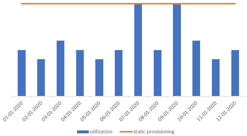
Figure 9.1 – Static provisioning for peak
The distance between the static, flat line and the top of the bar graph represents waste. We have 2 days of maximized utilization efficiency but inefficient usage (that is, waste) for the remainder of the days.
The elasticity of the cloud allows you to reduce this waste by provisioning resources you need when you need them. AWS uses the term auto scaling to represent the elastic provisioning of resources on demand to meet your system requirements. With elasticity, you achieve the efficiency that’s represented in the following screenshot. The difference between the provisioned line amount and the usage amount is lesser than the usage pattern in Figure 9.1 and shows better efficiency and less waste:
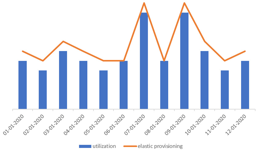
Figure 9.2 – Elastic provisioning matching supply with demand
AWS Auto Scaling is a service that helps you optimize your applications by supplying the resources you need, depending on your applications’ demands. The resources with AWS Auto Scaling can be EC2 instances, EC2 spot fleets, containers with Elastic Container Service (ECS), NoSQL databases such as DynamoDB, and AWS’ proprietary relational database service, Amazon Aurora. You define when you need these resources provisioned by a scaling policy.
Now that we’ve defined auto scaling, let’s see how AWS applies auto scaling to Amazon EC2 in various forms.
AWS Auto Scaling versus Amazon EC2 Auto Scaling
You can leverage resource-specific managed scaling such as Amazon EC2 Auto Scaling or AWS Auto Scaling to dynamically provision resources when needed. Both help to reduce waste because you only need (and pay) for those resources when your applications require them. Whereas resource-specific managed scaling applies only to said resources such as Amazon EC2, AWS Auto Scaling provides managed scaling for multiple resources across multiple services.
Let’s compare the two by looking at Amazon EC2 as a service. Amazon EC2 Auto Scaling optimizes your resource use by providing your application with the appropriate number of servers it needs to handle the required load. The service replaces unhealthy instances automatically, terminates instances when unneeded, and launches more (scales out) when required. You define how the service adds or removes instances by the policy.
You control scaling in one of two ways, as follows:
- The first is with manual scaling. You can scale manually, which involves monitoring your application and changing the configuration as needed. As a user, you can go into your Amazon EC2 auto-scaling fleet and make manual adjustments based on changes in demand in your environment.
- The other option is automatic scaling, which uses several AWS-provided scaling mechanisms through auto scaling. As humans, although we generally have good intentions, we are error-prone and tend to get bored of repetitive tasks. Auto scaling makes much more sense. The two types of automatic scaling are scheduled scaling and dynamic auto scaling. We’ll look at these two next:
- For predictive workloads, scheduled scaling can avoid delays due to extended startup times for EC2 instances. With scheduled scaling, we can evaluate historical runtimes to identify recurring scaling events such as scaling up at the beginning of the work week and scaling down as the work week ends. We can also take in individual events such as new product releases, new marketing campaigns, or special holiday deals that may drive an increase in traffic to our AWS environment. Amazon EC2 Auto Scaling takes care of launching and terminating resources based on our scaling policy’s predefined schedules.
- For unpredictable workloads, dynamic auto scaling fits the bill. Within dynamic auto scaling, there are three types, as outlined here:
- Simple scaling is the most elementary dynamic auto scaling type. With simple scaling, you must set a CloudWatch alarm to monitor a certain metric—say, central processing unit (CPU) utilization. If you set a policy such that when CPU utilization breaches a threshold of 80%, AWS is to add 20% more capacity, then auto scaling will perform this action when the application meets this condition. This is a very straightforward approach and doesn’t consider health checks or cooldowns. In other words, if an event occurred to launch 20% more capacity, the auto-scaling mechanism must wait for health checks on the new instances to complete and the cooldown on the scaling event to expire before it considers adding or removing instances. This might pose a problem, particularly when you experience sudden increases in load—you might not be able to afford to wait for these expiration times but need the environments to change rapidly.
- Step scaling is another policy that gives you more granular control. Rather than a blanket policy such as simple scaling, instead, you define different scaling events at different thresholds. In the preceding example, we said to provision 20% more capacity when CPU utilization is at 80%. With step scaling, you can use more granular metrics such as 10% more capacity when CPU utilization is between 60% and 70%, and 30% more capacity when CPU utilization is above 70%. Additionally, step scaling continues to respond to alarms even when a scaling activity or a health check is taking place. This makes step scaling more responsive than simple scaling.
- If we are to continue using CPU utilization as the defined scaling metric, then target tracking is the most convenient scaling policy that requires the least management. This is because, for step and simple scaling, you still have to create CloudWatch metrics and associate them with the policies, but for target tracking, Amazon EC2 Auto Scaling creates and manages CloudWatch alarms for you. With target tracking, you simply provide the desired application state, just like how you set your home thermostat to the desired temperature. Once set, the heating or cooling system will intermittently turn on/off to maintain that temperature. Similarly, a target tracking policy set at an aggregate average CPU utilization of 40% will ensure you have the optimal resources to maintain that target metric.
You can use Amazon EC2 Auto Scaling to manually or automatically scale your servers to meet your demand. Save your auto-scaling configurations in the form of launch templates. Launch templates make it easier for you to manage how your workloads automatically scale because you define the method in advance. In other words, launch templates are the what for when auto scaling occurs. Doing this drives efficiency and reduces waste because you only use the compute resources you need when you need them rather than overbuying to meet unexpected or expected demand.
CPU is a common metric when implementing auto scaling, but it’s not the only metric you can use. Many customers use memory, disk space, and network latency as metrics to trigger when an auto-scaling event should occur. You can even use your own custom metrics based on your workload requirements. For example, if you have a web application and want to use request-response error rates as the metric to scale more EC2 instances, then you can use a custom metric that counts for error rates and have Amazon EC2 Auto Scaling deploy more servers when your threshold has been breached.
Now, let’s see how AWS Auto Scaling relates to Amazon EC2 Auto Scaling.
When to use AWS Auto Scaling
Although the preceding example is specific to Amazon EC2, other services such as Amazon ECS, Amazon Aurora, and DynamoDB also have their own specific auto-scaling policies, which is why AWS Auto Scaling attempts to aggregate these disparate services into a unified interface where you can manage their scaling policies in one place.
AWS Auto Scaling supports only target-tracking scaling policies at the time of writing. Use AWS Auto Scaling if you intend to use target tracking because it is easier to manage and can also be used to set auto-scaling policies for other AWS services. Say you had a workload consisting of an auto-scaled group of EC2 instances, an Aurora cluster as a database, a spot fleet for batch processing, and were utilizing a target tracking metric. In that case, it would be more cumbersome to have to manage scaling for each service individually than managing them in one place through the AWS Auto Scaling service.
Predictive scaling leverages the capabilities of both AWS Auto Scaling and EC2 Auto Scaling, providing the ability to use ML models to analyze traffic over the past 14 days. Based on this historic data, predictive scaling identifies scheduled events for the next 2 days and then repeats the cycle every day to update your scheduled events based on the latest information available.
AWS Auto Scaling may simplify your auto-scaling needs across your AWS environment, but Amazon EC2 Auto Scaling gives you more control over your Amazon EC2 resources. Note that you don’t necessarily need to choose one or the other. You may choose AWS Auto Scaling for certain workloads that encompass various services, but when the need arises, you may use Amazon EC2 Auto Scaling to specify scaling policies for your Amazon EC2 fleet. Let’s move on to optimize other areas of our AWS environment—namely, within the analytics domain.
Optimizing analytics
If data is the new gold, we want to ensure we’re mining it without incurring waste. Data analytics and ML are discussion topics that deserve their own books but, in this section, we’ll summarize cost-optimization considerations when running these types of workloads. Broadly, we can categorize the steps involved as data ingestion, data exploration, model training, and model deployment.
We already know about Amazon S3 as an object store that functions nicely as a data lake. With data in S3, we can use a managed service such as Amazon Athena to run Structured Query Language (SQL) queries directly on our data in Amazon S3. Athena is serverless, meaning you don’t have to manage any infrastructure to run SQL queries on your data. Additionally, it scales automatically and parallelizes queries on large datasets without you having to specify configurations. It also requires no maintenance because the underlying servers powering Athena are managed by AWS. You pay for the query you run on Athena, thus optimizing data storage and minimizing query execution, which ensures lower costs.
Amazon Redshift is a data warehousing service on AWS that allows you to run complex analytic queries at a petabyte (PB) scale. These queries run on distributed and parallelized nodes. Unlike traditional relational databases, Redshift stores data in columns that are optimized for analytical applications, whereas it’s often the case to query based on aggregate summary statistics on columns. We’ll see an example of this in the next section.
For ML, Amazon SageMaker is a service that provides an ML platform for building, training, deploying, and monitoring ML models. SageMaker comes with a host of features that range from labeling data to monitoring a complete ML pipeline. With Amazon SageMaker, data scientists can launch ML-specific notebook instances (indicated by an ml. prefix) to prepare data, build ML models, and deploy them at scale. We’ll cover how to optimize ML compute using SageMaker in the next section.
Optimizing data ingestion and preparation
Data analytics starts with having data; you can’t get insights from data if you don’t have any, and you need a place to store that data. We’ve already discussed Amazon S3 Intelligent-Tiering in Chapter 7, Optimizing Storage, as an easy way to optimize storage costs by allowing AWS to manage the optimal storage class on our behalf.
We can also save on costs through the format in which we store our data. With Amazon S3, you are charged by the amount of storage, hence if we can find ways to minimize that storage amount, we can reduce our storage costs. Storing only the data that you need is always good to have in mind. It’s easy to create a data swamp out of a lake because you just never know if, and when, you’ll need a dataset. But instead of blindly putting all your data in Amazon S3 Standard or Intelligent-Tiering, try to understand your data’s access patterns, future needs, and business value. We may always intend to clean up our data afterward, but the more we put it off, the more data accumulates and the harder it becomes to comb through data to find what we actually need.
For data that you do need, use compression to save on storage space and pay less. Parquet is a popular columnar format for large-scale analytics workloads and can be used to save on storage costs but also save on query performance if you end up using AWS services such as Amazon Athena or Amazon Redshift. Values of a similar type such as string, data, and integer can be compressed and stored together, and because column values are stored together on disk, the query performance is more efficient.
The following screenshot shows a representation of columnar-based storage of a table. If you were to run a query on total views for Active users, you’d only need to query the ViewCount and UserStatus columns in a columnar store such as Redshift. This is much more efficient than having to query each row and read columns that you don’t need, as you would do in a traditional relational database:
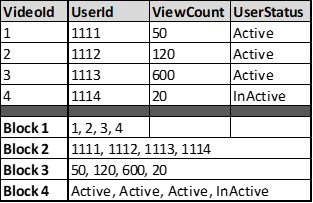
Figure 9.3 – Table with columnar-based storage
When using Athena, consider using a shared Amazon S3 location for query results. When setting up Athena, you must specify a location in S3 to store query results. By choosing a shared location, you can reuse cached query results, improve query performance, and save on data transfer costs. With Athena, you pay for the time it takes for the query to run. Hence, by minimizing the query execution time, you will be spending less. This is generally a good pattern, especially if you’re planning on using Athena to run ad hoc queries on your organization’s Cost and Usage Reports (CUR) data.
The following screenshot shows where you can manage these settings in the Amazon Athena console. Here, we specify the query result location (and optionally choose to encrypt) within the Query editor page.
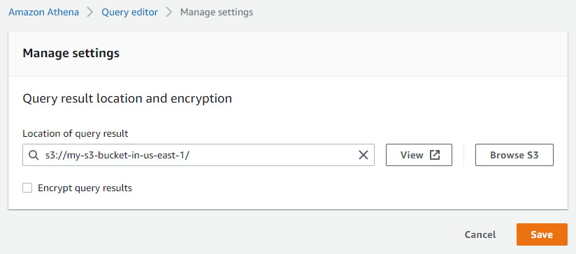
Figure 9.4 – Specifying Athena query results
We looked at Amazon Athena as an example service to run ad hoc queries. Another option is to use Amazon Redshift if you plan to run more complex joins and read workloads with long-running query times. Unlike Athena, you don’t pay per query with Redshift. Instead, you provision a cluster that is purpose-built for data warehousing-type workloads. You can also purchase Redshift RIs to save on costs for running steady-state, consistent Redshift clusters. Because we understand RI mechanics, let’s instead focus on optimizing the performance and cost of Redshift in how we use and operate the cluster.
You can leverage a feature of Amazon Redshift called concurrency scaling. This offers the ability to support scalable concurrent users and queries. When you enable concurrency scaling, Amazon Redshift automatically adds additional cluster capacity to specifically process read queries. When a Redshift cluster with concurrency scaling meets specific requirements such as Region location, node type, and node amount, queries can be routed to a concurrency-scaling cluster. You route queries to concurrency-scaling clusters by enabling a Workload Manager (WLM) queue.
Although you’re charged for concurrency-scaling clusters, you’re only charged for the time they’re in use. The concept here is similar to the auto-scaling discussion we had in the previous section. Consider provisioning a large Redshift cluster to meet high-performance requirements even if peak performance only occurs during a small percentage of the cluster’s lifetime. Usually, larger clusters equate to larger costs. If instead, you were able to leverage the dynamism of the cloud such as the concurrency-scaling feature of Redshift, you could meet your performance requirements, and only pay for it when needed.
In the following diagram, we see an example of concurrency scaling on Redshift in action. When a user initiates a query with concurrency scaling, the leader node of the main Redshift cluster receives the request and determines whether it fits the requirements for the concurrency-scaling queue. Redshift then sends the request to add the cluster depicted on the right side of the diagram. These two clusters constitute your concurrency cluster. As more queries arrive, they are sent to the concurrency-scaling cluster for processing. Optionally, we have Amazon S3, which stores the cluster’s snapshots, enabling the new concurrency cluster access by way of a caching layer. Finally, the results are delivered to the user through the response:
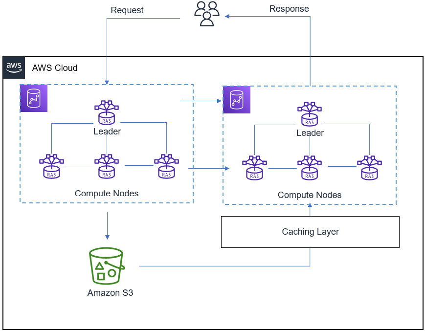
Figure 9.5 – Redshift concurrency scaling
Amazon Redshift also offers elastic resize options to resize your cluster quickly by adding nodes when your workload increases and removing nodes when demand decreases. This gives you some flexibility and comfort in knowing that you do not need to make the right decision upfront. You can iterate on your cluster’s configuration as your needs change. Elastic resizing automatically redistributes data to new nodes quickly when you resize using the same node type. Elastic resize can also change node types, whereby a snapshot is created and copied to a new node-type cluster.
An additional option for resizing your Redshift cluster is to use Amazon Redshift Spectrum. This feature of Redshift allows you to scale your data lake without needing to load data into the Redshift cluster. You can directly query data in Amazon S3 and join the data in S3 with Redshift. This saves you from having to duplicate storage costs in both services.
Lastly, because Amazon Redshift allows you to pause and later resume a cluster, be mindful of when a cluster is needed by teams. Although you can purchase RIs to save on cluster costs, if an always-on philosophy isn’t required for a workload, then save on costs by turning off the cluster. A practical exercise is to turn it off during weekends and holidays when you know teams or applications won’t need to be accessing your cluster. When a cluster is paused, on-demand billing is suspended, helping you to reduce waste.
We learned how you can optimize costs with Athena and Redshift in this section. Storing data efficiently by compressing it and leveraging columnar storage tools such as Redshift are ways to reduce the operational costs of using analytics services. We looked at some of Redshift’s features, focusing on elasticity to use and scale the service when you need to. In the next section, we’ll shift to the related but separate topic of ML. Because ML is often done after data preparation and data analysis, it logically fits as the next step in our data pipeline.
Optimizing ML
To uncover how we can optimize our ML costs, we must first understand which tasks constitute an ML workflow. We’ll look at the various steps involved in a typical ML process. Then, we’ll apply optimization methods to those specific steps using the various capabilities in AWS. We’ll focus on how you can optimize your model-training costs and model-deployment costs with Amazon SageMaker.
Understanding an ML workflow
An ML workflow typically requires data exploration and then feature engineering (FE) to transfer data to a format that can be used by an ML algorithm. The algorithm reads the data to find patterns and learns in a sense to generalize patterns so that it can predict outcomes on new, or unknown, data. This is often referred to as model training—you’re applying some mathematical algorithm that may be known and used popularly or something you created yourself to data that is proprietary to you or your organization. The application of an algorithm to your data creates an ML model. Then, you can apply this model to make predictions on new data. Amazon SageMaker is a fully managed platform that allows you to do just this.
SageMaker has tons of features that provide you with a unified platform to complete all tasks involved in an E2E ML workflow. This includes things such as data cleansing and preparation. Before you build an ML model, you need to format the data to remove unnecessary columns, remove missing values, change text columns to numeric values, and even add columns to define your features. Usually, you want to document all your steps into code to facilitate automation of these tasks in the form of a processing script so that you can run these data processing steps automatically and at scale.
You can use SageMaker Processing jobs to execute a processing script. Running these scripts can help you optimize because you only pay for the processing job for the duration of the task. An alternative could be to conduct your processing jobs in an Amazon EC2 instance if wanting to keep things in a cloud environment. However, this would require you to install all the necessary software on a fleet of instances for high availability (HA) and parallel processing, patch the instances, secure them, and right-size them, among other things. Rather than managing all this yourself, SageMaker Processing takes care of the resource provisioning, and data and artifact transfer, and terminates the resources once your job completes. Thus, you only pay for the resources used for the processing job while it runs. At the same time, you only need to use a relatively small SageMaker notebook instance to test and orchestrate your processing jobs.
Leveraging a fully managed service such as SageMaker helps you avoid unnecessary costs when it comes to managing and paying for compute resources for your ML workload. In line with our discussion from the beginning of this chapter, SageMaker helps you take advantage of AWS’ elasticity by having SageMaker manage your ML tasks’ infrastructure and paying for them only for the duration of the tasks’ runtime.
Important note
You may, however, choose to manage the infrastructure yourself if you find that you obtain a competitive advantage by doing so. Some companies have robust data science teams that have the knowledge and experience to manage their own ML infrastructure. They may even have the expertise to optimize that infrastructure at various levels such as code optimization, Savings Plans, and the use of open source software (OSS). If indeed you find better cost savings by managing your own ML workloads, then SageMaker may not be the right choice for you. However, we’ll continue the rest of this section assuming you chose SageMaker as your ML platform.
Let’s now move to the next step of the ML workflow and learn how to optimize our model-training tasks.
Optimizing model training and tuning
Because SageMaker decouples the ML development from task execution, you can easily adopt a pay-as-you-go model. For example, you can spin up a small, cheaper ml.t2.small instance to work on ML development tasks such as testing code, setting up configuration files, and defining your ML pipeline. You attach a SageMaker execution role to that instance with the required permissions to access datasets and then run the SageMaker Python SDK commands to run processing scripts, initiate training jobs, and deploy model endpoints.
At this point, you’re only paying for that ml.t2.small instance. You don’t necessarily want to train and deploy models on that instance because you’ll likely face out-of-memory (OOM) exceptions or other errors because of the computational- and memory-intensive requirements of model training. Rather than running resource-intensive training jobs on your ml.t2.small instance, you can elect to run training jobs on a separate, graphics processing unit (GPU)-based instance to optimize performance. SageMaker will spin up the resource required for your training job, and then spin down the instances when the job is complete. This allows you to only pay for the required resources when you need them, thereby reducing waste related to ML workloads.
At the same time, you don’t have to provision an expensive, GPU-based instance if you simply need it for data exploration and testing. SageMaker allows you to decouple training or processing jobs from experimentation. For example, the next code snippet shows a model-training job specifying that the training should be done on a single ml.m4.4xlarge instance. Even though the notebook instance used to instantiate and execute this code may be on an ml.t2.small instance, you gain the benefit of paying for the more expensive ml.m4.4xlarge instance only while the training job runs, while paying for a cheaper ml.t2.small instance for exploration. SageMaker will manage the training on your behalf and terminate it when the training job is complete, so you only pay for it while it runs.
In the following code snippet, we are calling the SageMaker estimator to train our model. We specify the container image we’d like to use, then the execution role that has permission to access the training data. Then, we specify the instance type and count to tell SageMaker which type of instance and how many of these instances to use for this training job:
model = sagemaker.estimator.Estimator(
container,
role,
train_instance_count=1,
train_instance_type='ml.m4.4xlarge,
sagemaker_session=sess)
That begs the following questions: What if my training jobs run a very long time? How can I ensure I’m not wasting valuable training time? SageMaker Debugger helps profile these job runs and provides recommendations to fix bottlenecks that may prolong unnecessarily long training jobs. Debugger can suggest things such as using a small instance based on lower GPU utilization or stopping training jobs early if subsequent training iterations are not improving the desired model metrics.
For example, training a deep learning (DL) model on a neural network (NN) usually involves adjusting weights on each training run (epoch) and observing the resulting model metrics. The network adjusts weights to see if those changes positively impact the model. However, there may come a point where adjusting the weights does not yield better results. If you are continuously running model-tuning jobs, but for every iteration it’s not improving your model, then it is wasteful to have those resources running. It’s better to early stop jobs to reduce unnecessary iterations. Early stopping can help reduce SageMaker training times, which correlate with your efforts to reduce waste.
You also have the option to use spot instances for training jobs, which may be appropriate for training jobs that can tolerate interruptions, or when using algorithms that support checkpointing (refer to Chapter 6, Optimizing Compute, for details on spot). You can specify the use of spot instances within the estimator by using the following code:
use_spot_instance=True.
Model = sagemaker.estimator.Estimator(
container,
role,
train_instance_count=1,
train_instance_type='ml.m4.4xlarge,
use_spot_instance=True,
max_wait = 120,
sagemaker_session=sess)
Because a spot instance may terminate before the training job completes, using the max_wait parameter will tell SageMaker to wait a certain number of seconds (in this case, 120 seconds) for new spot instances to replace terminated ones. Once the max_wait time passes, the job completes. If using checkpoints, the training job will commence from the latest checkpoint when the spot instances were terminated.
Another cost-reducing strategy is in the way we specify how data is made ready by SageMaker during training. By default, files are read using File mode, which copies all data to an instance when a training job starts. The alternative is to use Pipe mode, which loads data like a stream. Note that these modes do not appear on the screen as options to select; you must specify these as parameters.
Using File mode for large files (above 10 gigabytes (GB)) prevents a long pause at the start of a training job just to get the file loaded into SageMaker. Instead, by using Pipe mode, data will be streamed in parallel from S3 directly into a training run. This provides higher input/output (I/O) and allows the training job to start early and end faster, and ultimately reduces training-job costs. We can specify the use of Pipe mode through the input_mode configuration, as illustrated in the following code snippet:
model = sagemaker.estimator.Estimator(
container,
role,
train_instance_count=1,
train_instance_type='ml.m4.4xlarge,
input_mode='Pipe'…)
We looked at several ways to reduce your training costs on Amazon SageMaker. Leverage spot instances if you can tolerate interruption to pay for spare compute as a discount versus paying for on-demand instances for training. Additionally, consider using the Pipe input mode to ensure the training job ends sooner. Also, leverage built-in features such as SageMaker Debugger to help you identify ways to optimize your training configuration. Because you only pay for the resources for the duration of your training and tuning jobs, use these tools to ensure those jobs don’t take longer than necessary. Let’s move on to the next step of an ML workflow: the deployment phase.
Optimizing model deployment
Once you have a trained model, you can deploy them to SageMaker endpoints. These endpoints can be persistent for real-time online inference. Many customers create Hypertext Transfer Protocol Secure (HTTPS) endpoints that allow users and applications to request real-time inference for low-latency use cases. SageMaker will manage these endpoints on your behalf, including automatically scaling them on your behalf to meet demand. However, you will be paying for these endpoints on an hourly basis, depending on the instance type you choose for the endpoint. As you can imagine, the more endpoints you have running, the more your costs will increase.
Endpoints are long-running resources that are easy to leave running even if you may not have use for them. Let’s imagine you deploy a real-time ML model using a blue/green deployment. You have two identical model endpoints and, once ready, you cut over from the blue environment to the green environment. The green environment now serves 100% of inference requests through your endpoint while the blue environment sits idle. To remove unused SageMaker endpoints, we can apply the same discipline we used to remove stale Elastic Block Store (EBS) volumes, as discussed in Chapter 7, Optimizing Storage. CloudWatch alerts can help notify you when a SageMaker endpoint is not receiving invocation requests. For example, use the Invocations metric to get the total number of requests sent to a model endpoint using Sum statistics. If you see zero invocations consistently, it may be a good time to delete the endpoint.
There may be more than one EC2 instance up and running behind a SageMaker endpoint serving predictions using SageMaker hosting services. Therefore, the more endpoints you have, the more costs you will incur. Although SageMaker Savings Plans can help offset the costs, it’s also wise to minimize the number of endpoints to remove unnecessary costs.
If you have similar models that can serve predictions through a shared serving endpoint, consider using SageMaker multi-model endpoints to avoid paying for additional endpoints. Multi-model endpoints are a scalable and cost-efficient solution to deploying several models while minimizing the cost of paying for endpoints. These models share a container that can host multiple models. This not only reduces cost, but also the administrative requirement of you having to manage multiple models across multiple endpoints.
For example, you may have a model that predicts home prices for a geographic region in the US. Home prices vary based on location. You may have a model that serves distinct predictions for homes in New York versus homes in Texas and other locations. You can place all these models under a single endpoint and invoke a location-specific model based on the request.
Multi-model endpoints are useful when similar models can be served without needing to access all the models at the same time. You can invoke a specific model by specifying the target model name as a parameter in the prediction request, as shown in the next diagram.
Here, we see a multi-model endpoint with two models, model_1 and model_2. SageMaker automatically serves the model based on the TargetModel parameter specified in the invoke_endpoint method. SageMaker will route the inference request to the instance behind the endpoint and will download the model from the Amazon S3 bucket that holds the model artifacts:
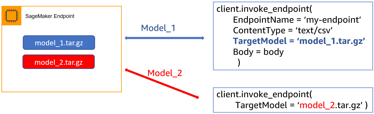
Figure 9.6 – SageMaker multi-model endpoint
Although SageMaker provides a variety of instance types for processing, model training, and deployment, sometimes you may not be able to find quite the right size. GPU instances are appropriate for model training on large datasets, but they can typically be oversized for smaller-batch inference requests.
By attaching an Elastic Inference Accelerator (EIA), you can boost your instance with a GPU-based add-on. This provides you the flexibility to choose a base CPU instance and dynamically add GPUs with the EIA until you find the right specification you require for your inference needs. This helps you optimize your base resources such as CPU and random-access memory (RAM) while keeping GPUs lower but having the flexibility to add GPUs when needed, all while saving costs. The following code snippet shows you how to add an ml.eia2.medium instance to an ml.m4.xlarge instance when deploying a SageMaker model:
predictor = model.deploy(
initial_instance_count=1,
instance_type='ml.m4.xlarge',
accelerator_type='ml.eia2.medium')
SageMaker also offers Savings Plans such as EC2 Instance and Compute Savings Plans. We unpacked a lot of how Savings Plans work in Chapter 6, Optimizing Compute, and their mechanisms are similar in how they are applied to SageMaker usage. You still specify a term length and payment option (no upfront, partial upfront, or all upfront). However, unlike EC2 Savings Plans, SageMaker Saving Plans only have one discount rate, meaning you cannot choose between instance-specific Savings Plans (such as EC2 Instance Savings Plans) and Compute Savings Plans.
The following screenshot shows how to select a SageMaker Savings Plan in Cost Explorer. You simply select a term (1 or 3 years), an hourly commitment, and a payment option:
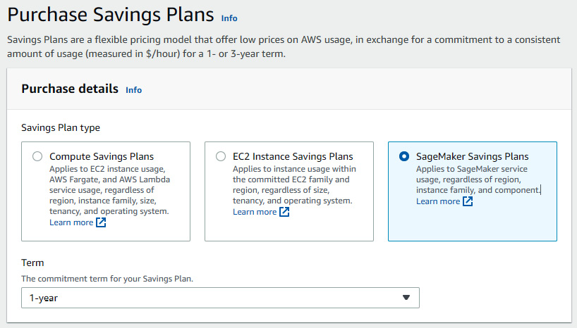
Figure 9.7 – SageMaker Savings Plans
SageMaker Savings Plans apply to all eligible Regions and SageMaker components. Whether you use SageMaker Processing, training, hosting, or just a notebook instance for testing, the Savings Plan commitment will apply to these components to help you save as an organization. And as with EC2 Savings Plans, if your usage of SageMaker exceeds your Savings Plan commitment, that usage will be charged the on-demand rate.
We covered optimization considerations for deploying ML models using Amazon SageMaker. We learned about SageMaker endpoint hygiene to ensure we’re not paying for persistent endpoints unnecessarily. We also learned about multi-model endpoints to reduce the cost of paying for multiple endpoints. Finally, we learned about the applicability of SageMaker Savings Plans to cover our ML workloads.
Summary
In this chapter, we covered topics that went beyond compute, storage, and networking. We saw how to apply cost-optimization methods for more advanced cloud-native environments including analytics and ML.
We unpacked AWS elasticity and what that means for architecting our workload. Take advantage of auto-scaling tools on AWS. These tools themselves are free. You only pay for the resources provisioned by scale-out activities and benefit by not paying for terminated resources from scale-in events. You learned about the various scaling policies and the difference between AWS Auto Scaling and Amazon EC2 Auto Scaling.
We then explored the realm of analytics. We found ways to optimize costs using compression, setting up the right data structure, and Redshift concurrency-scaling and workload management features.
Lastly, we learned about the various steps in a typical ML workload. We looked at ways to optimize data processing jobs using a managed service such as Amazon SageMaker. We also looked at optimization strategies for training and tuning jobs by leveraging spot instances, SageMaker Debugger, and file input modes. Then, we found optimization opportunities in model deployment using multi-model endpoints, elastic inference, and SageMaker Savings Plans.
We covered many topics in this section, focusing on the tactical work to optimize your cloud environments. In the next and final part of the book, we’ll learn about operationalizing these tasks in ways to optimize at scale as your organization grows. We’ll also focus on the people aspect of cost optimization and the importance of people, processes, and communication so that cost optimization doesn’t become a one-time activity but a continuous discipline that yields long-term results for your organization.
Further reading
For more information, refer to the following links:
- AWS Auto Scaling, 2022: https://aws.amazon.com/autoscaling/
- Amazon EC2 Auto Scaling, 2022: https://aws.amazon.com/ec2/autoscaling/
- Predictive scaling for Amazon EC2 Auto Scaling, 2022: https://docs.aws.amazon.com/autoscaling/ec2/userguide/ec2-auto-scaling-predictive-scaling.html
- Athena compression support, 2022: https://docs.aws.amazon.com/athena/latest/ug/compression-formats.html
- Working with concurrency scaling, 2022: https://docs.aws.amazon.com/redshift/latest/dg/concurrency-scaling.html
- Implementing workload management, 2022: https://docs.aws.amazon.com/redshift/latest/dg/cm-c-implementing-workload-management.html
- Host multiple models in one container behind one endpoint, 2022: https://docs.aws.amazon.com/sagemaker/latest/dg/multi-model-endpoints.html
- Monitor Amazon SageMaker with Amazon CloudWatch, 2022: https://docs.aws.amazon.com/sagemaker/latest/dg/monitoring-cloudwatch.html#cloudwatch-metrics-endpoint-invocation
- Processing, 2022: https://sagemaker.readthedocs.io/en/stable/api/training/processing.html#module-sagemaker.processing