7

Working with Lists and Maps

We have worked with lists and maps in earlier chapters in various queries. But we have not discussed how lists and maps can make Cypher queries more powerful. They are first-class types in Cypher, like string and integer, and can make it easy to build complex queries. This chapter discusses how we can handle both lists and maps as input and output. We will discuss how we can prepare lists from data, iterate lists to process data, handle nested maps, and return map projections.

The following aspects will be covered in this chapter:

• Working with lists
• Working with maps

We will be covering lists first. We will discuss in detail how lists work in Cypher and explore various ways we can manipulate and work with lists, both as input and output. We will also look at different types of lists and the functions available to work with them.

Let’s get onto working with lists.

Working with lists

Lists are the core data type in Cypher and because of this, there is extensive support for lists in Cypher. Lists hold elements in a sequence so that we can iterate the list in any order. They can hold any type of value. All of the elements in a list can be of the same type: whether integer, string, map, or list. It is also possible to mix and match different types in the same list.

We will take a look at different aspects of lists, such as using them as input and building lists for output or intermediate processing, along with using various built-in functions to process lists in this section.

Working with basic list capabilities

Cypher lists can be used to hold any type of data, including integers, strings, and so on. They hold the data in sequence like an array but are not limited to a single type. We can use indexing to access content or leverage built-in functions from Cypher to access data.

Let’s take a look at an example:

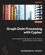
WITH [1,2,3,4] as intList, ['test1', 'test2', 'test3'] as strList
RETURN intList[0] as intValue, strList[0] as strValue

This code snippet shows how a list can hold different types of data objects:

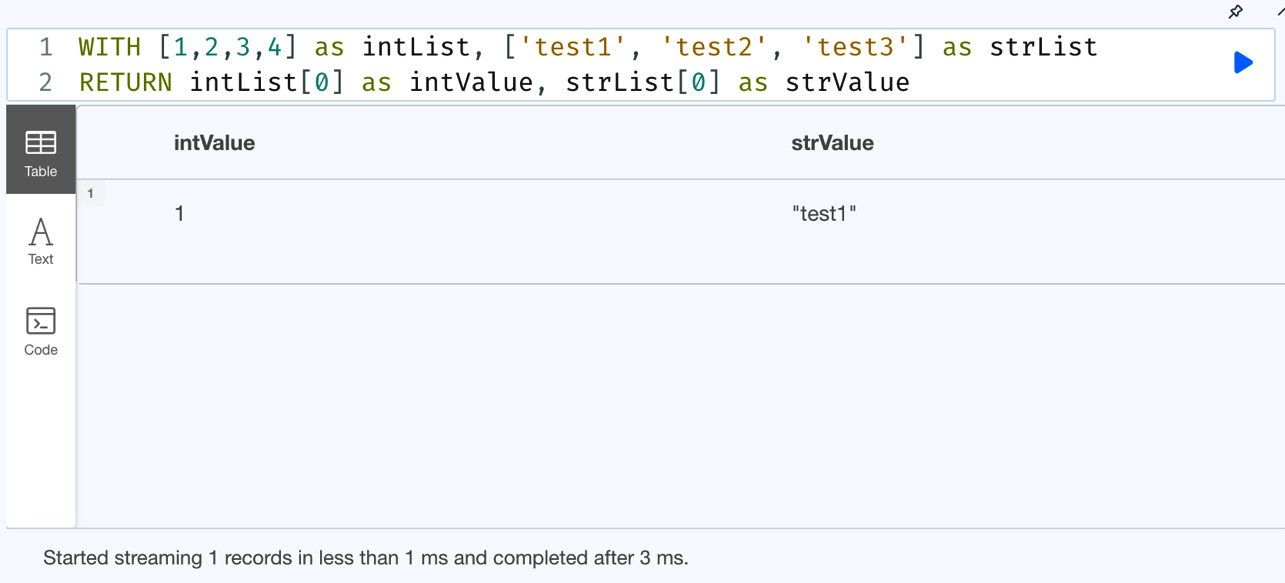
Figure 7.1 – Basic list usage

From the screenshot, we can see the usage of an integer list and a string list. When we access the values from the list, we get the appropriately typed value returned.

It is also possible for a list to contain multiple types of data objects. Let’s take a look at an example:

WITH [1,2,3,4] as intList, ['test1', 'test2', 'test3'] as strList
RETURN intList+strList as final

In this code snippet, we are attempting to combine an integer list and a string list.

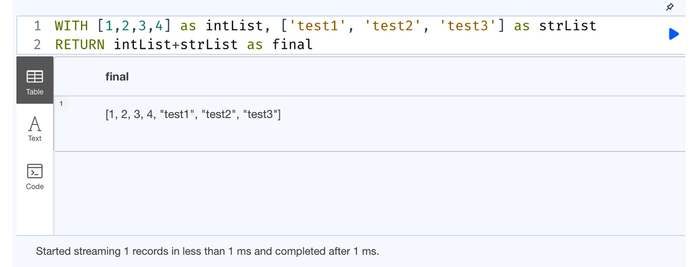
Figure 7.2 – Combining lists with different data types

From the previous screenshot, we can see that when we combine an integer list and a string list, we get a single list with both types of data objects.

It is also possible to have lists as elements in a list. Let’s look at an example:

WITH [1,2,[10,11],3,4] as list
RETURN list[0] as e1, list[2] as e2

We can see in the previous code snippet that we have a list embedded in another list.

Let’s run this in the browser to see what the response looks like:

Figure 7.3 – A list embedded in another list

From the screenshot, we can see when we refer to element 0, we get an integer value, and element 2 returns the embedded list.

Next, let’s take a look at list operators.

Working with list operators

In this section, we will discuss list operators along with their usage.

First, let’s take a look at the + operator. This operator concatenates one or more lists:

WITH [1,2,3,4] as list1, [2,3,5] as list2
RETURN list1+list2 as final

This code concatenates two lists and creates a single list that contains all the elements in the order they are appended.

Let’s execute it in the browser to see what the response looks like:

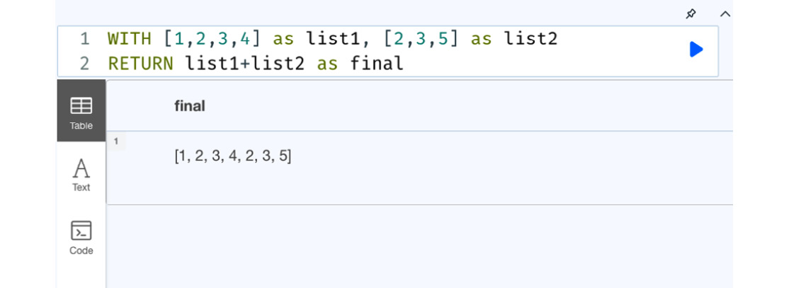
Figure 7.4 – Concatenating two lists

We can see from the screenshot that a single list is created by concatenating two lists. We can also see that it does not remove any duplicates from the list.

It is also possible to concatenate lists with multiple types to create a single list with objects with different data types. We have seen this already in Figure 7.2.

Let’s look at the IN operator next.

The IN operator lets us check whether a given value is in the list or not. Let’s look at an example usage:

WITH [1, 2, 3, 4, 5] as list
UNWIND list as n
WITH n
WHERE n IN [2,4,8]
RETURN n

The preceding code snippet shows the usage of the IN operator. From given a list of numbers, it checks whether the number is in another list and returns the matching numbers.

Let’s execute it in the browser to see what the response looks like:

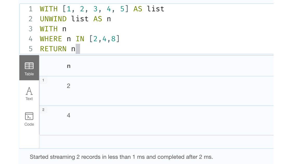
Figure 7.5 – Usage of the IN operator

The screenshot shows the usage of the IN operator and the query response.

It is also possible to look for the existence of list values using the IN operator. Let’s look at this example:

WITH [1,2,3,[11,12], 3,4] as list
RETURN [2, 1] IN list as wrong, [11,12] in list as right

This code snippet shows how to check for the existence of a list in another list.

Let’s execute it in the browser to see what the response looks like:

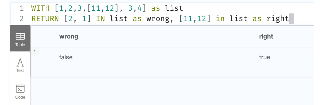
Figure 7.6 – Usage of the IN operator to check for lists

The screenshot shows the usage of the IN operator to check for the existence of a list in another list and the response.

We will take a look at the [ ] index operator next.

You can access the elements of a list using the [ ] operator. Let’s look at a few examples:

WITH [1,2,3,[11,12], 3,4] as list
RETURN list[0] as e1

This code segment shows how to return the first element in a list.

Let’s execute it in the browser to see what the response looks like:

Figure 7.7 – Accessing the first element of the list using the [ ] operator

We can see from the screenshot that it returns the first element of the list.

You can also use the value -1 to get the last element of a list without knowing the size of the list:

WITH [1,2,3,[11,12], 3,4] as list
RETURN list[-1] as e1

This code snippet shows how to get the last element in a list.

Let’s execute it in the browser to see what the response looks like:

Figure 7.8 – Accessing the last element of the list using the [ ] operator

The screenshot shows we got the last element using -1 as the index value.

The indexing continues with negative values with indexing starting from -1 and traversing backward with each value going backward. Let’s look at an example of this usage:

WITH [1,2,3,[11,12], 3,4] as list
RETURN list[-1] as last, list[-2] as prevLast

This code snippet shows how a -1 index gives us the last element and a -2 index gives us the element that is before the last element.

Let’s execute it in the browser to see what the response looks like:

Figure 7.9 – Accessing the last element of the list using the [ ] operator and negative indices

From the screenshot, we can see the negative index values traverse the list from the last element to the first. This gives us easier means to iterate the list from first to last or last to first.

When we try to access the list beyond its length, the [ ] operator returns a null value.

Let’s look at an example of this:

WITH [1,2,3,[11,12], 3,4] as list
RETURN size(list) as length, list[10] as e

This code snippet returns the list length and the 10th element of the list, which is beyond the length of the list.

Let’s execute it in the browser to see what the response looks like:

Figure 7.10 – The [ ] operator usage beyond list length

From the screenshot, we can see that the list length is 6, and when we try to access the 10th element, we get a null value as the response.

It is also possible to use the index operator by using a dynamic parameter. Let’s look at an example of this:

:param index=>1;
WITH [1,2,3,[11,12], 3,4] as list
RETURN list[$index] as e

This code segment shows two queries. You would need to execute them one by one to see the response in the browser:

1. First, the :param statement needs to be executed. This is a browser directive to define parameterized variables.
2. Then, execute the next two lines that use the parameter we defined earlier.

Let’s execute it in the browser to see what the response looks like:

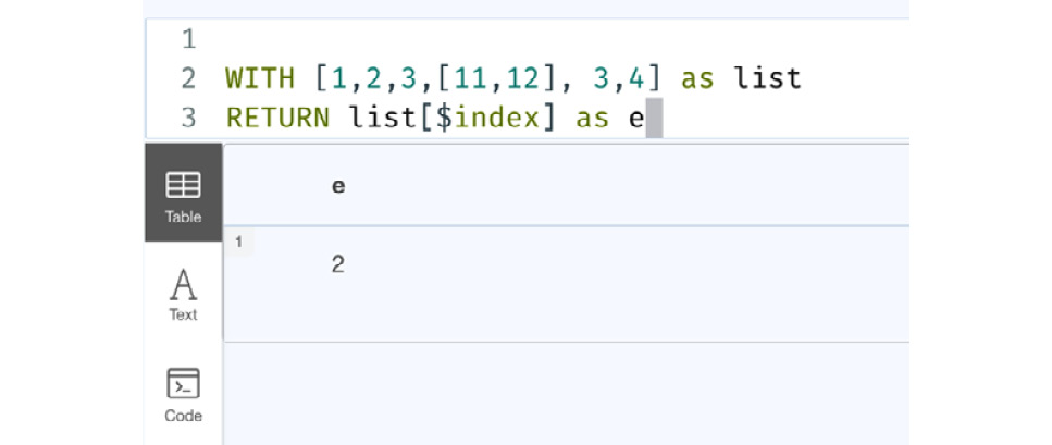
Figure 7.11 – Using a parameterized variable as an index for the list

From the screenshot, we can see that we are getting the first element as the response when we used $index as the index value since we defined its value as 1 beforehand.

Next, we will revisit all the list functions we worked with in earlier chapters. This will give us a more comprehensive understanding of lists.

Revisiting the list functions

In this section, we will revisit the list functions we worked with in earlier chapters:

• The range function provides a way to create a list with numbers. It takes a start value, an end value, and an optional step parameter and returns a list of all integer values bound by start and end. The syntax of the range function is as follows:

  range(start, end [, step])

The step value is optional. When step is not provided, it defaults to 1. If you provide a negative step value, this function returns an empty list. A sample usage of the range function would be as follows:

RETURN range(1,10)

This returns a list with values from 1 to 10 in increments of 1. Let’s review the head function next.

• The head function returns the first element of the list:

  WITH [1,2,3,4] as list

  RETURN head(list)

This returns a value of 1, which is at the head of the list. Let’s review the tail function next.

• The tail function returns a list with all the elements except the first element of the list:

  WITH [1,2,3,4] as list

  RETURN tail(list)

This returns a list with the values 2,3, and 4 in it. Let’s review the last function next.

• The last function returns the last element in the list:

  WITH [1,2,3,4] as list

  RETURN last(list)

This returns a value of 4, which is the last element in the list. Let’s review the size function next.

• The size function returns the size of the list:

  WITH [1,2,3,4,10,15] as list

  RETURN size(list)

This returns a value of 6, which is the length of the list. Let’s review the reverse function next.

• The reverse function returns the list in reverse order:

  WITH [1,2,3,4,10,15] as list

  RETURN reverse(list)

This returns a list that reads [15, 10, 4, 3, 2, 1], which is the original list in reverse order. Let’s review the reduce function next.

• The reduce function is used to aggregate a result by traversing a list. This function goes through each item in the list and passes it to an expression and the resultant value is assigned to an intermediate variable. Once all the items in the list are processed, the final value is returned.

The syntax of this function looks as follows:

reduce(accumulator = initial, variable IN list | expression)

The following table explains the arguments of the function.

Table 7.12 – The reduce function’s parameters

Let’s take a look at an example query that uses this function:

WITH [1,2,3,4,10,15] as list
RETURN reduce(sum=0, x in list | sum + x) as total

This returns the sum of all the values in the list, which is 35.

Next, we will take a look at COLLECT and UNWIND.

Working with COLLECT and UNWIND

COLLECT and UNWIND are the means to build a list or iterate a list and perform a set of operations.

The COLLECT function allows data to be collected into a list. Let’s look at an example of this:

MATCH (d:Drug)
WITH d
LIMIT 10
RETURN COLLECT(d.code)

This query returns the codes of 10 drugs as a list.

Let’s execute it in the browser to see what the response looks like:

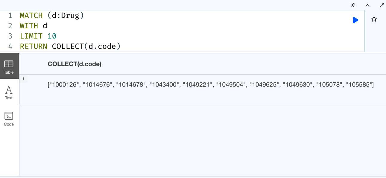
Figure 7.13 – Basic COLLECT usage

We can see from the screenshot that the response contains the list with the drug codes as a single value returned.

UNWIND is a Cypher clause that can convert a list into rows so that it can be processed one row at a time.

Let’s start with a basic usage first:

WITH [1,2,3,4] as list
UNWIND list as e
RETURN e

This query converts a list into rows and returns each row.

Let’s execute it in the browser to see what the response looks like:

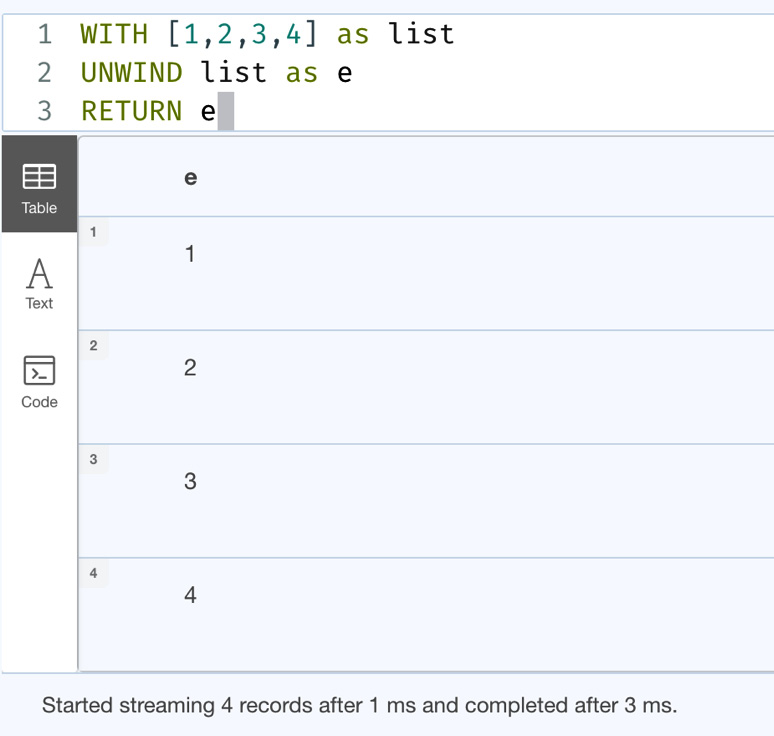
Figure 7.14 – Basic UNWIND usage

From the screenshot, we can see that we have four rows returned, one row for each element in the list.

Let’s take a look at another example where there are duplicates in the list:

WITH [1,2,3,3,4] as list
UNWIND list as e
RETURN e

This query returns five rows as there are duplicates in the data. We can combine the DISTINCT clause with UNWIND to work with unique rows of data.

Let’s look at this aspect:

WITH [1,2,3,3,4] as list
UNWIND list as e
RETURN DISTINCT e

This query returns only the distinct values from the list.

Let’s execute it in the browser to see what the response looks like:

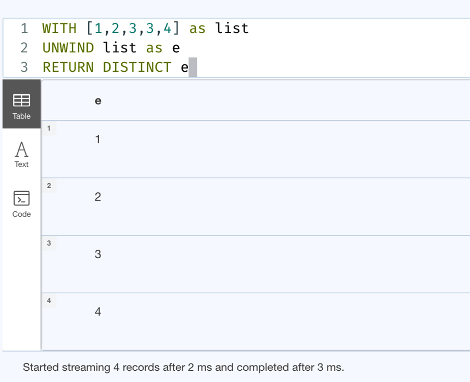
Figure 7.15 – Combining UNWIND with DISTINCT

From the screenshot, we can see that the response contains only four rows, while there are five elements in the list.

It is also possible to use UNWIND along with any expression that returns a list. Let’s look at an example of this:

WITH [1,2] as list1, [3,4] as list2
UNWIND (list2+list1) as e
RETURN e

This query creates a new list by combining two lists and performs UNWIND on it.

Let’s execute it in the browser to see what the response looks like:

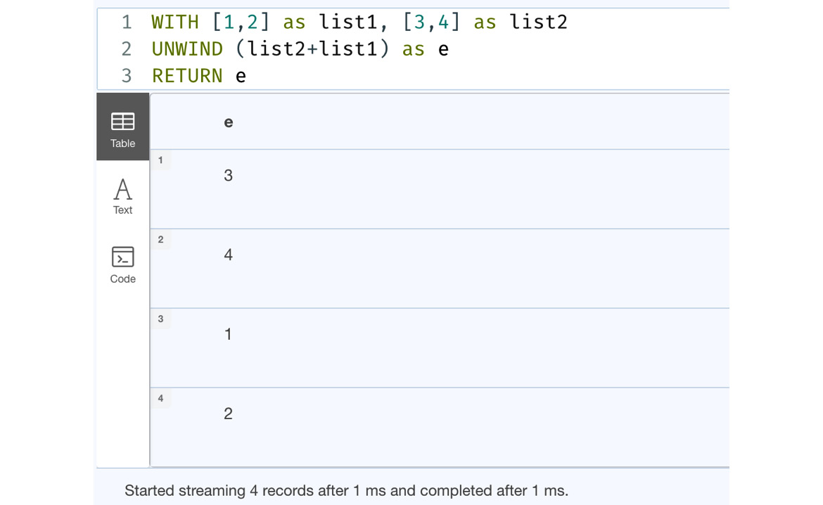
Figure 7.16 – Using list expressions with UNWIND

From the screenshot, we can see that list2 and list1 are combined first and UNWIND returns the rows of the combined list values.

It is also possible to work with nested lists using UNWIND. Let’s look at an example of this:

WITH [[1,2], [3,4]] as list
UNWIND list as inner
UNWIND inner as e
RETURN e

With nested lists, you also need to nest the UNWIND statements to process them as shown in the preceding query.

Let’s execute the preceding code in the browser to see what the response looks like.

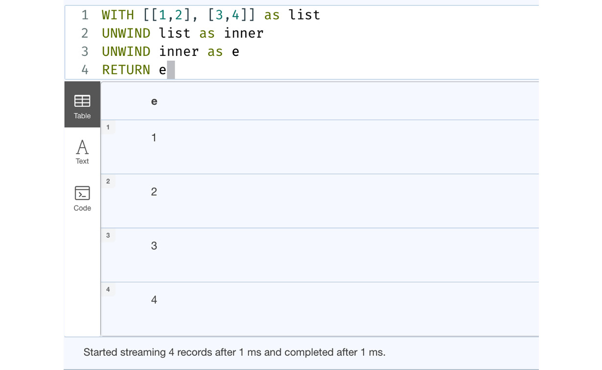
Figure 7.17 – Handling nested lists with UNWIND

We can see from the screenshot that we iterated the nested list and got all the individual elements from all the inner lists.

Now that we have taken a look at the various aspects of lists in Cypher, we will take a look at working with maps in Cypher next.

Working with maps

In this section, we will take a look at working with maps in Cypher. Maps in Cypher represent key-value pairs. The keys must be strings and values can be any object. Maps can be defined in Cypher inline, where they are called literal maps, or they can be passed as parameters. Every node and relationship object can also be treated as a map in Cypher, so that we can access all the properties using dot (.) notation or index ([ ]) notation.

A map is like a JavaScript Object Notation (JSON) object. A sample JSON object looks like this:

{
  "firstName": "John",
  "lastName": "Smith",
  "isAlive": true,
  "age": 27
}

If we represented the same map in Cypher, it would look like this:

WITH {
  firstName: "John",
  lastName: "Smith",
  isAlive: true,
  age: 27
} as map
RETURN map

We can see from the code that the keys in this map representation are not enclosed by double quotes as they are being represented as JSON. These are called literal maps in Cypher.

Let’s execute it in the browser to see what the response looks like.

Figure 7.18 – Map representation in Cypher

As we can see from the preceding screenshot, while in Cypher we are not using double quotes for keys, in the data returned there are double quotes for keys, which is exactly what the actual JSON object looks like.

In Cypher, this is called a literal map. These literal maps can be as simple as the ones we have seen in the preceding figure, or they can be complex nested objects. Let’s look at an example:

WITH {
  firstName: "John",
  lastName: "Smith",
  isAlive: true,
  age: 27,
  address: {
    line1: "1 address ln",
    city: "Newark",
    state: "NJ",
    country: "USA"
  },
  aliases: ["Johny", "John"]
} as map
RETURN map.firstName, map.lastName, map.address.state, map.aliases[0]

We can see that in this map object that we have a nested map and a list of values in the outer map. Also, in the RETURN statement, we can see that we are able to refer to the keys in the map using the dot notation, similar to how JSON objects are used.

Let’s execute it in the browser to see what the response looks like.

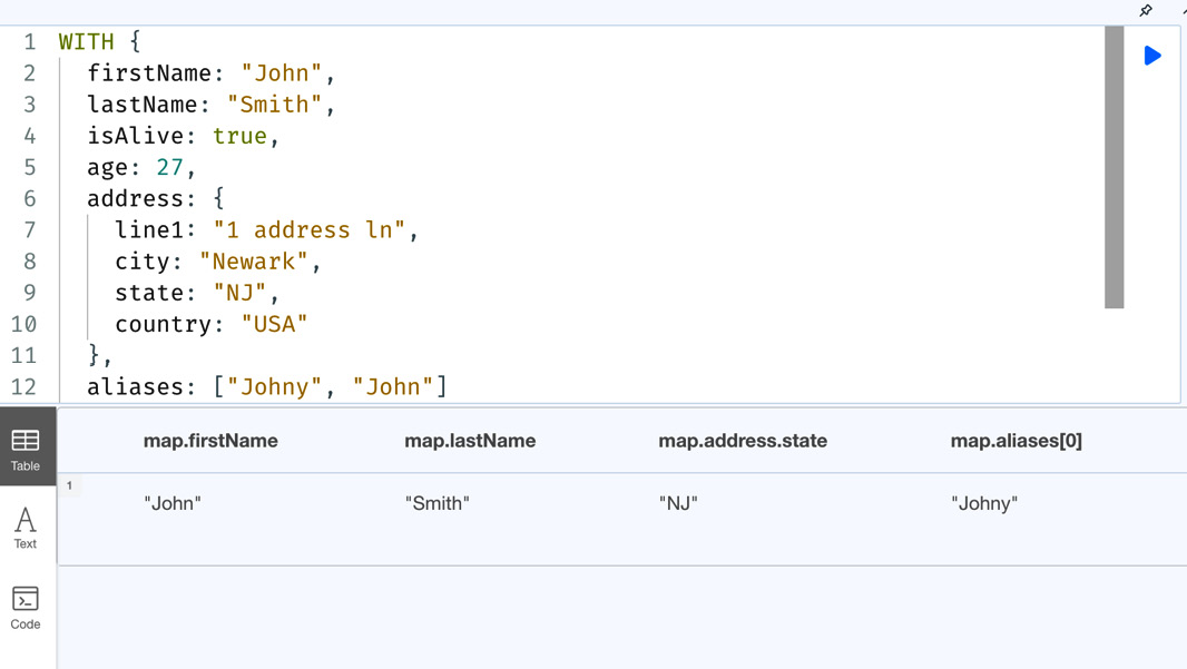
Figure 7.19 – Nested map usage in Cypher

From the screenshot, we can see that the values from the map related to the keys referred are returned. We can also see that not only can we get values of basic types that are accessible directly from the map, such as firstName and lastName, but we can also access nested content, such as a state key from the address object in the source map, along with the first element of the list identified by the aliases key.

In the previous query, we access the values using dot notation. We can also retrieve values using the [ ] syntax. Let’s take a look at this:

WITH {
  firstName: "John",
  lastName: "Smith",
  isAlive: true,
  age: 27,
  address: {
    line1: "1 address ln",
    city: "Newark",
    state: "NJ",
    country: "USA"
  },
  aliases: ["Johny", "John"]
} as map
RETURN map["firstName"], map["lastName"], map["address"]["state"], map["aliases"][0]

We can see in the preceding query that we are able to access the values using the [ ] syntax.

Let’s execute it in the browser to see what the response looks like.

Figure 7.20 – Map value access using the [ ] syntax

We can see that the response is the same for accessing values from the map using dot notation or the [ ] syntax. This syntax is more useful when there are special characters or spaces in the key names. In that case, dot notation cannot be used to refer to those keys as it would cause syntax errors. Index notation can help us to avoid this issue and still be able to access the map values.

One more thing to note in Cypher is that for string literals, you can either use double quotes or single quotes.

Now, let’s look at how we can work with map projections of data in Cypher.

Working with map projections

Cypher provides a concept called map projections. Map projections are a very useful tool to build a simple response from node or relationship entities to return only the content we need. They are maps built using nodes, relationship properties, and other values.

Let’s take a look at an example of this:

MATCH (d:Drug)
WITH d
LIMIT 10
RETURN d{.code, .description, label: labels(d)[0]}

This query will retrieve the first 10 drug nodes and create a map projection with the code and description properties for the Drug node and the first label of that node.

Let’s execute it in the browser to see what the response looks like.

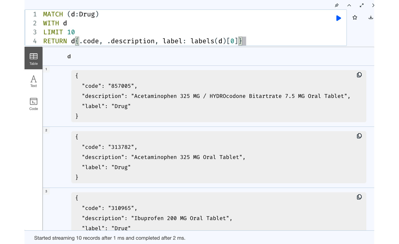
Figure 7.21 – Using map projections from Cypher

From the screenshot, we can see that the response is rows of maps with the codes, descriptions, and labels we built in the query. The response returned is a simple map with values and not a node entity.

Let’s take a look at another simpler usage of map projections:

MATCH (d:Drug)
WITH d
LIMIT 10
RETURN d{.*}

This returns only the properties of the drug nodes as a map, and not all the other metadata associated with the node. This kind of usage is very useful when we don’t need all the node metadata.

Let’s execute it in the browser to see what the response looks like.

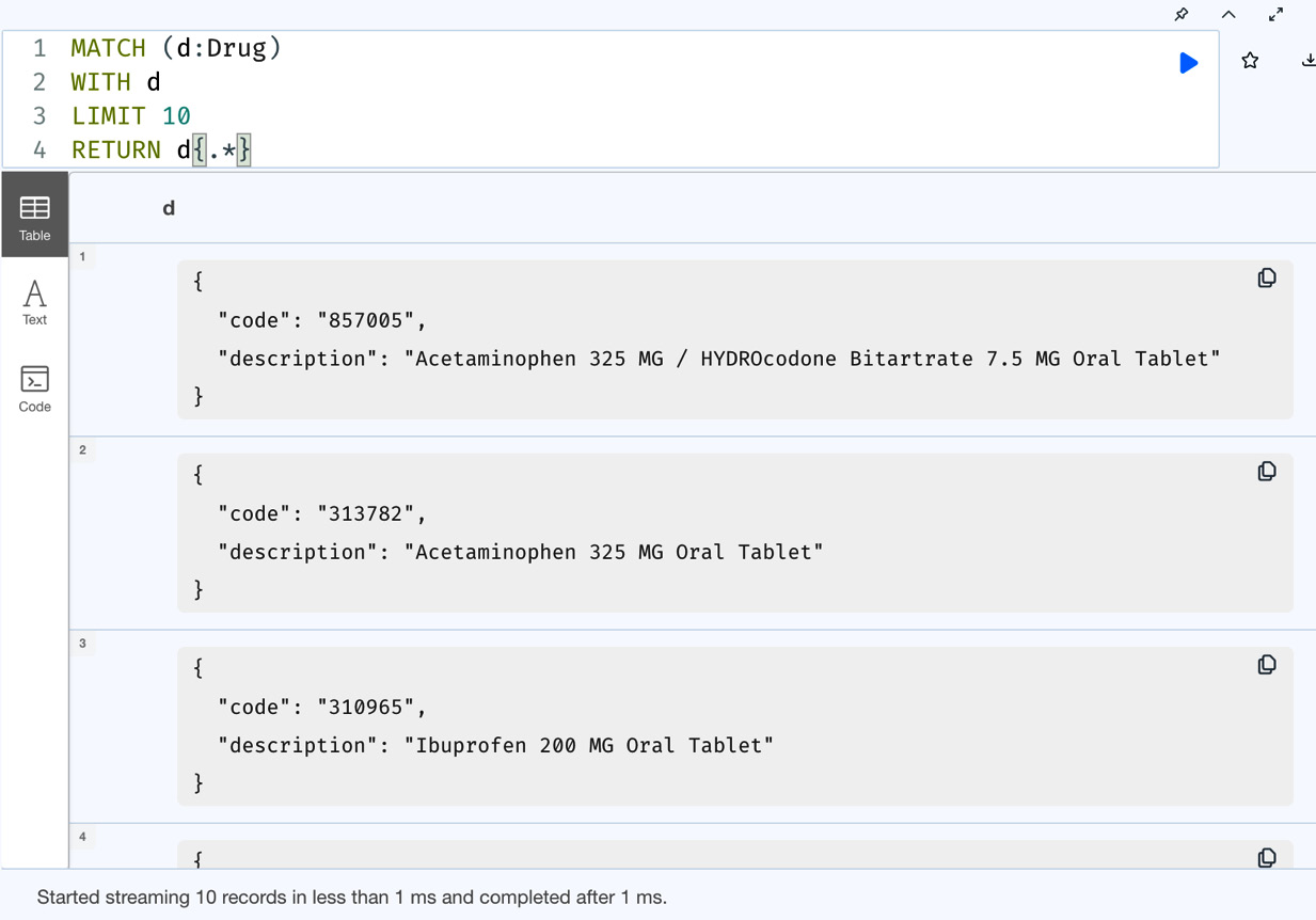
Figure 7.22 – Basic map projections of node properties

From the screenshot, we can see that we have just the properties of the node as a map projection. There is no node metadata returned here.

For reference purposes, let’s take a look at what the response would have been if we returned the node:

MATCH (d:Drug)
WITH d
LIMIT 10
RETURN d

This query returns the node.

Let’s execute it in the browser to see what the response looks like.

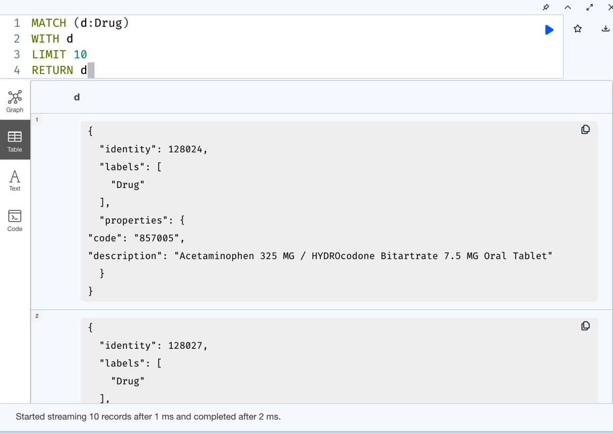
Figure 7.23 – Node data return data for comparison

From the screenshot, we can see that when we return the node, we get the node identity labels as the list along with properties as a separate map. This could be very useful for graph visualizations, but for basic applications that are interested only in the property content, using map projections can reduce the network traffic and be more efficient.

Now, let’s look at working with lists and maps together.

Combining lists and maps

Most of the time when we are loading batch data, we use lists of maps as data input to Cypher. We saw this in Chapter 3, Loading Data with Cypher, when we were loading data using LOAD CSV.

LOAD CSV turn each row in the CSV file into a map and we then process each row. Let’s review this:

LOAD CSV WITH HEADERS from "file:///data.csv" AS row
WITH row
MERGE (p:Person {id:row.id})
SET p.firstName = row.firstName,
p.lastName = row.lastName

Here, the LOAD CSV clause reads the CSV file and converts each line into a map value and assigns it to a variable named row. We process one line at a time, which is the map assigned to the variable named row in the next steps of the query. Since the list of values in the line is converted into a map, we can access the values in the map using dot notation. In this query, we are accessing the keys, which are part of CSV headers, such as id, firstName and lastName. We will get one row object per line in the CSV file, excluding the header line, and we process in sequence one row at a time. If there are 100 lines in the CSV, then the last three lines of code will be executed 100 times.

If the same data is being sent as a parameter to the query using the driver, then the query will look like this:

UNWIND $data as row
WITH row
MERGE (p:Person {id:row.id})
SET p.firstName = row.firstName,
p.lastName = row.lastName

The $data variable holds the list of maps. We are unwinding the list to process one record at a time.

Now that we have taken a deeper look at how maps can be consumed, let’s look at a summary of what we covered in this chapter.

Summary

In this chapter, we have looked at how lists and maps are core data types in Cypher for data manipulation and processing data. We looked at creating basic lists, how they can store different data types, and how we can access data using operators and functions. Also, we looked at how maps work in Cypher and how to use them when we are returning data. We also looked at how LOAD CSV creates a map for each row to be processed. Also, we took a look at lists of maps that are provided by applications using the driver to be processed to ingest data similar to LOAD CSV.

In the next chapter, we will take a deep dive into advanced querying using WITH, FOREACH, CASE, and other Cypher clauses.