7

Using Simulation to Improve and Optimize Systems

Simulation models allow us to obtain a lot of information using few resources. As often happens in life, simulation models are also subject to improvements to increase their performance. Through optimization techniques, we try to modify the performance of a model to obtain improvements both in terms of the results and when trying to exploit resources. Optimization problems are usually so complex that a solution cannot be determined analytically. Complexity is determined first by the number of variables and constraints, which define the size of the problem, and then by the possible presence of nonlinear functions. To solve an optimization problem, it is necessary to use an iterative algorithm that, given a current approximation of the solution, determines—with an appropriate sequence of operations—and updates this approximation. Starting from an initial approximation, a sequence of approximations that progressively improve the solution is determined.

In this chapter, we will learn how to use the main optimization techniques to improve the performance of our simulation models. We will learn how to use the gradient descent technique, the Newton-Raphson method, and stochastic gradient descent. We will also learn how to apply these techniques with practical examples.

In this chapter, we’re going to cover the following main topics:

• Introducing numerical optimization techniques
• Exploring the gradient descent technique
• Understanding the Newton-Raphson method
• Deepening our knowledge of stochastic gradient descent
• Approaching the Expectation-Maximization (EM) algorithm
• Understanding Simulated Annealing (SA)
• Discovering multivariate optimization methods in Python

Technical requirements

In this chapter, we will learn how to use simulation models to improve and optimize systems. To deal with the topics in this chapter, it is necessary that you have a basic knowledge of algebra and mathematical modeling. To work with the Python code in this chapter, you’ll need the following files (available on GitHub at the following URL: https://github.com/PacktPublishing/Hands-On-Simulation-Modeling-with-Python-Second-Edition):

• gradient_descent.py
• newton_raphson.py
• gaussian_mixtures.py
• simulated_annealing.py
• scipy_optimize.py

Introducing numerical optimization techniques

In real life, optimizing means choosing the best option among several available alternatives. Each of us optimizes an itinerary to reach a destination, organize our day, determine how we use savings, and so on. In mathematics, optimizing means determining the value of the variables of a function so that it assumes its minimum or maximum. Optimization is a discipline that deals with the formulation of useful models in applications, thereby using efficient methods to identify an optimal solution.

Optimization models have great practical interest for the many applications offered. In fact, there are numerous decision-making processes that require you to determine a choice that minimizes the cost or maximizes the gain and is, therefore, attributable to optimization models. In optimization theory, a relevant position is occupied by mathematical optimization models, for which the evaluation function and the constraints that characterize the permissible alternatives are expressed through equations and inequalities. Mathematical optimization models come in different forms:

• Linear optimization
• Integer optimization
• Nonlinear optimization

Defining an optimization problem

An optimization problem consists of trying to determine the points that belong to a set F in which a function f takes values that are as low as possible. This problem is represented in the following form:

Here, we have the following:

• f is called the objective function
• F is called the feasible set and contains all the admissible choices for x

Important note

If you have a maximization problem—that is, if you have to find a point where the function f takes on the highest possible value, you can always go back to the minimal problem, thus changing the sign of the objective function.

The elements that minimize the function f by satisfying the previous relationship are called global optimal solutions, also known as optimal solutions or minimum solutions. The corresponding value of the objective function f is called the global optimum value, also known as the optimal or minimum.

The complexity of the optimization problem—that is, its difficulty of resolution—obviously depends on the characteristics of the objective function and the structure of the flexible set. Usually, an optimization problem is characterized by whether there is complete freedom in the choice of the vector x. We can therefore state that there are two types of problems, as follows:

• Unconstrained minimization problem, if F = Rn; that is, if the flexible set F coincides with the whole set Rn
• Constrained minimization problem, if F ⊂ Rn; that is, if the flexible set F is only a part of the set Rn

When trying to solve an optimization problem, the first difficulty we face is understanding if it is well placed, in the sense that there may not be a point of F where the function f (x) takes the value pi as small. In fact, one of the following conditions could occur:

• The flexible set F may be empty
• The flexible set F may not be empty but the objective function could have a lower limit equal to −∞
• The flexible set F may not be empty and the objective function could have a lower limit equal to −∞ but also, in this case, there could be no global minimum points of f on F

A sufficient but not necessary condition for the existence of a global minimum point in an optimization problem is that expressed by the Weierstrass theorem through the following proposition: let F ⊂ Rn be a non-empty and compact set. Let f be a continuous function on F. If so, a global minimum point of f exists in F.

The previous proposition applies only to the class of constrained problems in which the flexible set is compact. To establish existence results for problems with non-compact flexible sets—that is, in the case where F = Rn—it is necessary to try to characterize some subset of F containing optimal solutions to the problem.

Important note

A compact space is a topological space where every open covering of it contains a finished sub-covering.

In general, there isn’t always an optimal solution for the problem at hand, and, where it exists, it isn’t always unique.

Explaining local optimality

Unfortunately, all global optimality conditions have limited application interest. In fact, they are linked to the overall behavior of the objective function on the admissible set and, therefore, are necessarily described by complex conditions from a computational point of view. Next to the notion of global optimality, as introduced by defining the optimization model, it is appropriate to define the concept of local optimality.

We can define a local optimum as the best solution to a problem in a small neighborhood of possible solutions. In the following diagram, we can identify four local minimum conditions for the function f (x), which therefore represent the local optimum:

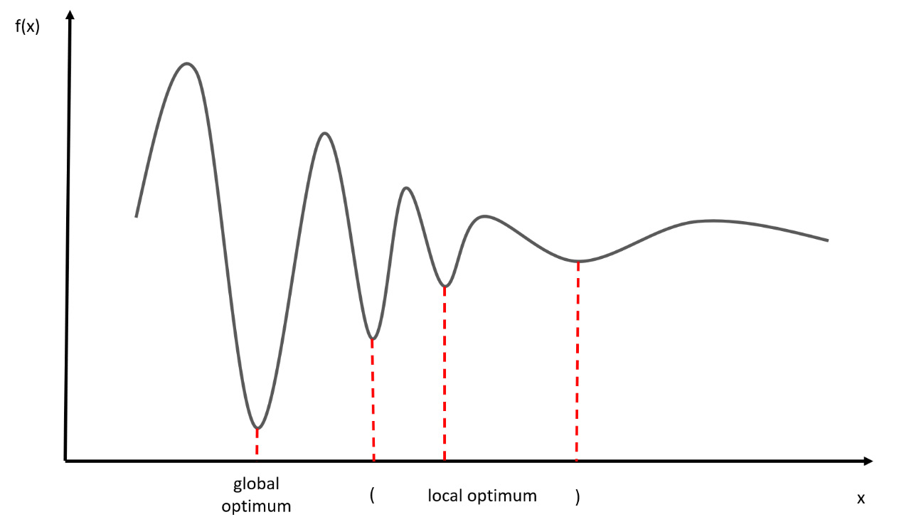
Figure 7.1 – Local minimum conditions for the f(x) function

However, only one of these is a global optimum, while the other three remain local optimums. Local optimality conditions are more useful from an application point of view. These are nothing but necessary conditions, but in general, they are not sufficient. This is because an assigned point is a local minimum point of a minimization problem. Therefore, from a theoretical point of view, they do not give a satisfactory characterization of the local minima of the optimization problem, but they do play an important role in the definition of minimization algorithms.

Many problems that are faced in real life can be represented as nonlinear optimization problems. This motivates the increasing interest, from a technical and scientific point of view, toward the study and development of methods that can face and solve this class of difficult mathematical problems.

Let’s now see the most widely used optimization technique.

Exploring the gradient descent technique

The goal of any simulation algorithm is to reduce the difference between the values predicted by the model and the actual values returned by the data. This is because a lower error between the actual and expected values indicates that the algorithm has done a good simulation job. Reducing this difference simply means minimizing the objective function that the model being built is based on.

Defining descent methods

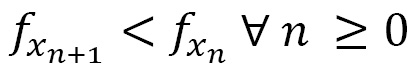
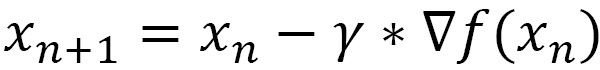
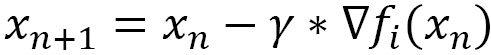
Descent methods are iterative methods that, starting from an initial point x0 ∈ Rn, generate a sequence of points {xn} n ∈ N defined by the following equation:

Here, the vector is a search direction and the scalar is a positive parameter called step length, which indicates the distance by which we move in the direction.

In a descent method, the vector and the parameter are chosen to guarantee the decrease of the objective f function at each iteration, as follows:

Using the vector, we take a direction of descent, which is such that the line x = xn + forms an obtuse angle with the gradient vector ∇f (xn). In this way, it is possible to guarantee the decrease of f, provided that is sufficiently small.

Depending on the choice of there are different descent methods. The most common are these methods:

• Gradient descent method
• Newton-Raphson method

Let’s start by analyzing the gradient descent algorithm.

Approaching the gradient descent algorithm

A gradient is a vector-valued function that represents the slope of the tangent of the function graph, indicating the direction of the maximum rate of increase of the function. Let’s consider the convex function represented in the following diagram:

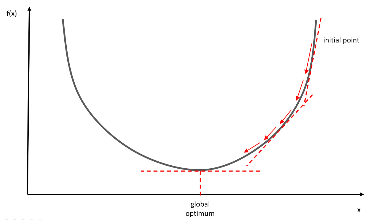
Figure 7.2 – The convex function

The goal of the gradient descent algorithm is to reach the lowest point of this function. In more technical terms, the gradient represents a derivative that indicates the slope or inclination of the objective function.

To understand this better, let’s assume we got lost in the mountains at night with poor visibility. We can only feel the slope of the ground under our feet. Our goal is to reach the lowest point of the mountain. To do this, we will have to walk a few steps and move toward the direction of the highest slope. We will do this iteratively, moving one step at a time until we finally reach the mountain valley.

In mathematics, the derivative is the rate of change or slope of a function at a given point. So, the value of the derivative is the slope of the slope at a specific point. The gradient represents the same thing, with the addition that it is a vector value function that stores partial derivatives. This means that the gradient is a vector and that each of its components is a partial derivative with respect to a specific variable.

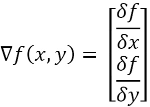
Let’s analyze a function, f (x, y)—that is, a two-variable function, x and y. Its gradient is a vector containing the partial derivatives of f: the first with respect to x and the second with respect to y. If we calculate the partial derivatives of f, we get the following:

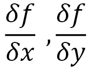
The first of these two expressions is called a partial derivative with respect to x, while the second partial derivative is with respect to y. The gradient is the following vector:

The preceding equation is a function that represents a point in a two-dimensional space, or a two-dimensional vector. Each component indicates the steepest climbing direction for each of the function variables. Hence, the gradient points in the direction where the function increases the most in.

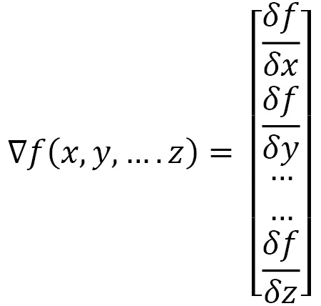
Similarly, if we have a function with five variables, we would get a gradient vector with five partial derivatives. Generally, a function with n variables results in an n-dimensional gradient vector, as follows:

For gradient descent, however, we don’t want to maximize f as fast as possible. Instead, we want to minimize it—that is, find the smallest point that minimizes the function.

Suppose we have a function y = f (x). Gradient descent is based on the observation that if the function f is defined and differentiable in a neighborhood of x, then this function decreases faster if we move in the direction of the negative gradient. Starting from a value of x, we can write the following:

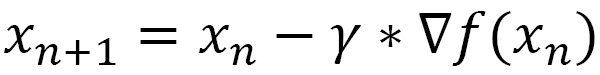
Here, we have the following:

• is the learning rate
• is the gradient

For sufficiently small values, the algorithm converges to the minimum value of the function f in a finite number of iterations.

Important note

Basically, if the gradient is negative, the objective function at that point is decreasing, which means that the parameter must move toward larger values to reach a minimum point. On the contrary, if the gradient is positive, the parameters move toward smaller values to reach the lower values of the objective function.

Understanding the learning rate

The gradient descent algorithm searches for the minimum of the objective function through an iterative process. At each step, an estimate of the gradient is performed to direct the descent in the direction that minimizes the objective function. In this procedure, the choice of learning rate parameter becomes crucial. This parameter determines how quickly or slowly we will move to the optimal values of the objective function:

• If it is too small, we will need too many iterations to converge to the best values
• If the learning rate is very high, we will skip the optimal solution

In the following diagram, you can see the two possible scenarios imposed by the value of the learning rate:

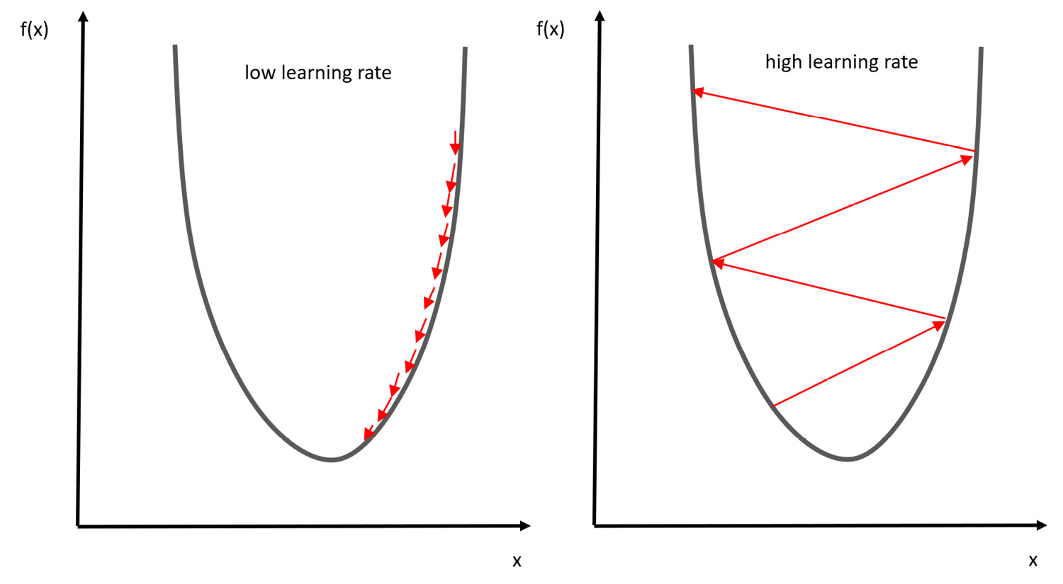
Figure 7.3 – Scenarios for the learning rate

Due to this, it is essential to use a good learning rate. The best way to identify the optimal learning rate is through trial and error.

Explaining the trial and error method

The term trial and error defines a heuristic method that aims to find a solution to a problem by attempting it and checking if it has produced the desired effect. If so, the attempt constitutes a solution to the problem; otherwise, we continue with a different attempt.

Let’s analyze the essential characteristics of the method:

• It is oriented toward the solution: It does not aim to find out why an attempt works, but simply seeks it.
• It is specific to the problem in question: It has no claim to generalize to other problems.
• It is not optimal: It usually limits itself to finding a single solution that will usually not be the best possible one.
• It does not require having a thorough knowledge of it: It proposes to find a solution to a problem of which little or nothing is known.

The trial and error method can be used to find all solutions to the problem or the best solution among them if there is more than one. In this case, instead of stopping at the first attempt that provided the desired result, we take note of it and continue in the attempts until all the solutions are found. In the end, these are compared based on a given criterion, which will determine which of them is to be considered the best.

Implementing gradient descent in Python

In this section, we will apply what we have learned so far on gradient descent by completing a practical example. We will define a function and then use that method to find the minimum point of the function. As always, we will analyze the code line by line:

1. Let’s start by importing the necessary libraries:

   import numpy as np

   import matplotlib.pyplot as plt

numpy is a Python library that contains numerous functions that help us manage multidimensional matrices. Furthermore, it contains a large collection of high-level mathematical functions we can use on these matrices.

matplotlib is a Python library for printing high-quality graphics. With matplotlib, it is possible to generate graphs, histograms, bar graphs, power spectra, error graphs, scatter graphs, and so on with a few commands. It is a collection of command-line functions, like those provided by MATLAB.

2. Now, let’s define the function:

   x = np.linspace(-1,3,100)

   y=x**2-2*x+1

First, we defined an interval for the dependent variable x. We will only need this to visualize the function and draw a graph. To do this, we used the linspace() function. This function creates numerical sequences. Then, we passed three arguments: the starting point, the ending point, and the number of points to be generated. Next, we defined a parabolic function.

3. Now, we can draw a graph and display it:

   fig = plt.figure()

   axdef = fig.add_subplot(1, 1, 1)

   axdef.spines['left'].set_position('center')

   axdef.spines['bottom'].set_position('zero')

   axdef.spines['right'].set_color('none')

   axdef.spines['top'].set_color('none')

   axdef.xaxis.set_ticks_position('bottom')

   axdef.yaxis.set_ticks_position('left')

   plt.plot(x,y, 'r')

   plt.show()

First, we defined a new figure and then set the axes so that the x axis coincides with the minimum value of the function and the y axis coincides with the center of the parabola. This will make it easier to visually locate the minimum point of the function. The following diagram is printed:

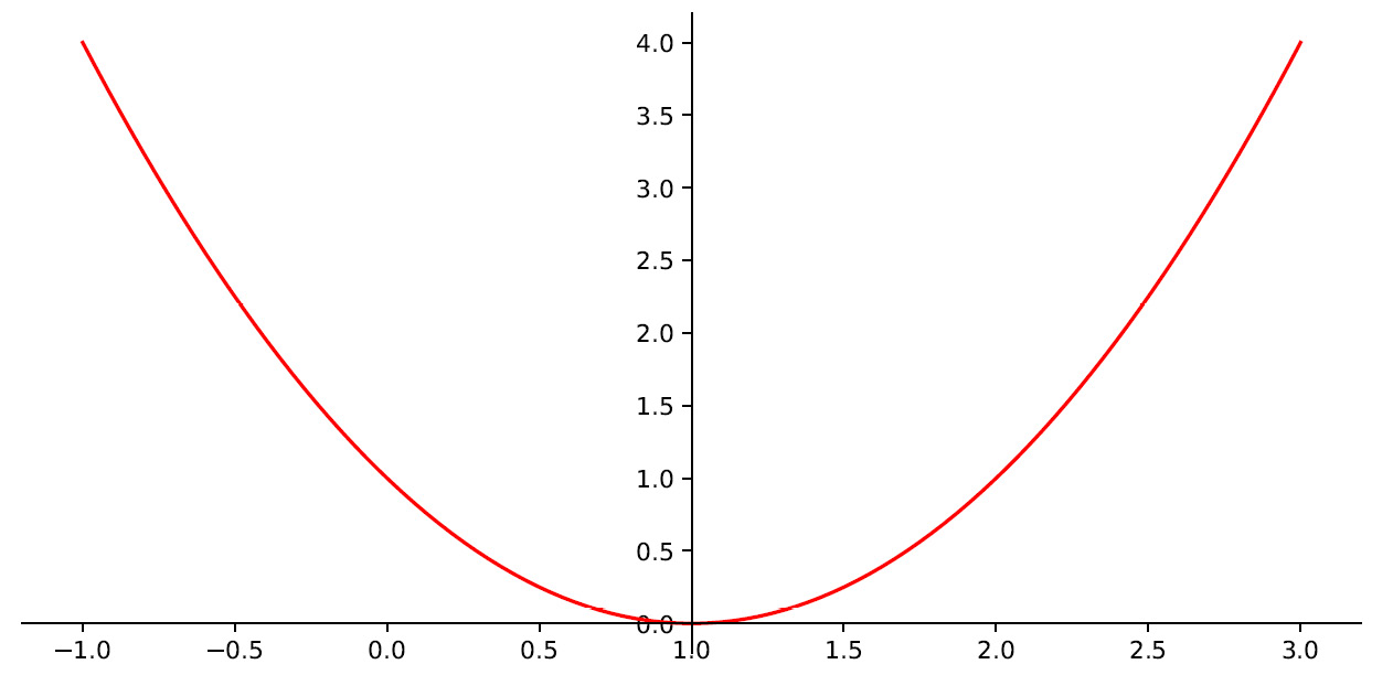
Figure 7.4 – The minimum point of the function

As we can see, the minimum point of the function corresponding to y = 0 occurs for a value of x equal to 1. This will be the value that we will have to determine through the gradient descent method.

4. Now, let’s define the gradient function:

   Gradf = lambda x: 2*x-2  

Recall that the gradient of a function is its derivative. In this case, doing this is easy since it is a single-variable function.

5. Before applying the iterative procedure, it is necessary to initialize a series of variables:

   actual_X  = 3 

   learning_rate  = 0.01 

   precision_value = 0.000001 

   previous_step_size = 1 

   max_iteration = 10000 

   iteration_counter = 0 

So, let’s describe in detail the meaning of these variables:

• The actual_X variable will contain the current value of the independent variable x. To start, we initialize it at x = 3, which represents the far-right value of the display range of the function in the graph.
• The learning_rate variable contains the learning rate. As explained in the Understanding the learning rate section, it is set to 0.01. We can try to see what happens if we change that value.
• The precision_value variable will contain the value that defines the degree of precision of our algorithm. Being an iterative procedure, the solution is refined at each iteration and tends to converge. But this convergence may come after a very large number of iterations, so to save resources, it is advisable to stop the iterative procedure once adequate precision has been reached.
• The previous_step_size variable will contain the calculation of this precision and will be initialized to 1.
• The max_iteration variable contains the maximum number of iterations that we have provided for our algorithm. This value will be used to stop the procedure if it does not converge.
• Finally, the iteration_counter variable will be the iteration counter.

6. Now, we are ready for the iteration procedure:

   while previous_step_size  > precision_value  and iteration_counter  < max_iteration :

       PreviousX = actual_X 

       actual_X  = actual_X  - learning_rate  * Gradf(PreviousX) 

       previous_step_size  = abs(actual_X  - PreviousX) 

       iteration_counter  = iteration_counter +1 

       print("Number of iterations = ",iteration_counter ,"
   Actual value of x  is = ",actual_X ) 

       print("X value of f(x) minimum = ", actual_X ) 

The iterative procedure uses a while loop, which will repeat itself until both conditions are verified (TRUE). When at least one of the two assumes a FALSE value, the cycle will be stopped. The two conditions provide a check on the precision and the number of iterations.

This procedure, as anticipated in the Defining descent methods section, requires that we update the current value of x in the direction of the gradient’s descent. We do this using the following equation:

At each step of the cycle, the previous value of x is stored so that we can calculate the precision of the previous step as the absolute value of the difference between the two x values. In addition, the step counter is increased at each step. At the end of each step, the number of iterations and the current value of the x are printed, as follows:

Number of iterations =  520 
Actual value of x  is =  1.0000547758790321
Number of iterations =  521 
Actual value of x  is =  1.0000536803614515
Number of iterations =  522 
Actual value of x  is =  1.0000526067542224
Number of iterations =  523 
Actual value of x  is =  1.000051554619138
Number of iterations =  524 
Actual value of x  is =  1.0000505235267552
Number of iterations =  525 
Actual value of x  is =  1.0000495130562201
Number of iterations =  526 
Actual value of x  is =  1.0000485227950957

As we can see at each step, the value of x progressively approaches the exact value. Here, 526 iterations were executed.

7. At the end of the procedure, we can print the result:

   print("X value of f(x) minimum = ", actual_X )

The following result is returned:

X value of f(x) minimum =  1.0000485227950957

As we can verify, the returned value is very close to the exact value, which is equal to 1. It differs precisely from the value of the precision that we imposed as the term for the iterative procedure.

After analyzing in detail a practical case of application of the optimization technique based on the gradient descent method, we will now turn to the Newton-Raphson method, an iterative method to calculate the zeros of a function.

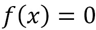
Understanding the Newton-Raphson method

Newton’s method is the main numerical method for the approximation of roots of nonlinear equations. The function is linearly approximated at each iteration to obtain a better estimate of the zero point.

Using the Newton-Raphson algorithm for root finding

Given a nonlinear function f and an initial approximation x0, Newton’s method generates a sequence of approximations {xk} k> 0 by constructing, for each k, a linear model of the function f in a neighborhood of xk and approximating the function with the model itself. This model can be constructed starting from Taylor’s development of the function f at a point x belonging to a neighborhood of the iterated current point xk, as follows:

Truncating Taylor’s first-order development gives us the following linear model:

The previous equation remains valid in a sufficiently small neighborhood of xk.

Given x0 as the initial data, the first iteration consists of calculating x1 as the zero value of the previous linear model with k = 0—that is, to solve the following scalar linear equation:

The previous equation leads to the next iterated x1 in the following form:

Similarly, the subsequent equation iterates x2, where x3 is constructed so that we can elaborate on a general validity equation, as follows:

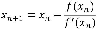
The form of the update equation is like the generic formula of descent methods. From a geometric point of view, the previous update equation represents the line tangent to the function f at the point (xk, f(xk)). It is for this reason that the method is also called the tangent method.

Geometrically, we can define this procedure through the following steps:

• The tangent of the function is plotted at the starting point x0.
• The intercept of this line is identified with the x axis. This point represents the new value x1.
• This procedure is repeated until convergence.

The following diagram shows this procedure:

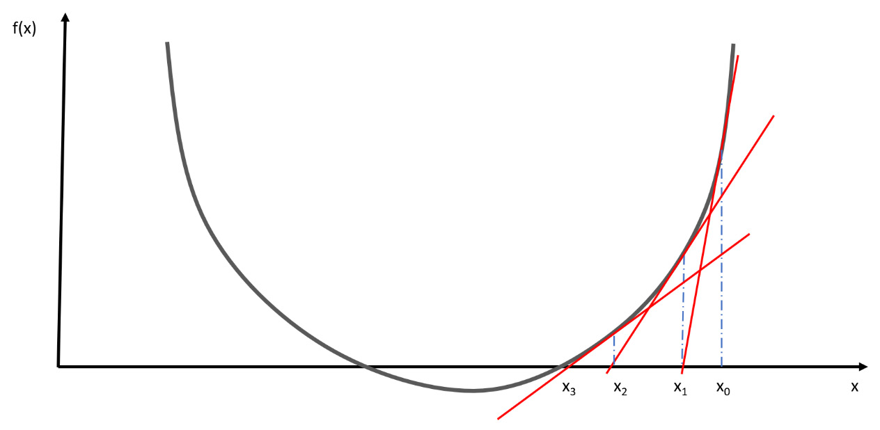
Figure 7.5 – The procedure of finding a tangent

This algorithm is well-defined if f’(xk) = 0 for every k. With regard to the computational cost, it can be noted that, at each iteration, the evaluation of the function f and its derivative before in point xk is required.

Approaching Newton-Raphson for numerical optimization

The Newton-Raphson method is also used for solving numerical optimization problems. In this case, the method takes the form of Newton’s method for finding the zeros of a function but is applied to the derivative of the function f. This is because determining the minimum point of the function f is equivalent to determining the root of the first derivative f′. The root of the first derivative is an optimality condition.

In this case, the update formula takes the following form:

In the previous equation, we have the following:

• is the first derivative of the function f
• is the second derivative of the function f

Important note

The Newton-Raphson method is usually preferred over the descending gradient method due to its speed. However, it requires knowledge of the analytical expression of the first and second derivatives and converges indiscriminately to the minima and maxima.

There are variants that bring this method to global convergence and that lower the computational cost by avoiding having to determine the direction of the research with direct methods.

Applying the Newton-Raphson technique

In this section, we will apply what we have learned so far about the Newton-Raphson method by completing a practical exercise. We’ll define a function and then use that method to find the minimum point of the function. As always, we will analyze the code line by line:

1. Let’s start by importing the necessary libraries:

   import numpy as np

   import matplotlib.pyplot as plt
2. Now, let’s define the function:

   x = np.linspace(0,3,100)

   y=x**3 -2*x**2 -x + 2

First, we defined an interval for the dependent variable x. We will only need this to visualize the function in order to draw a graph. To do this, we used the linspace() function. This function creates numerical sequences. Then, we passed three arguments: the starting point, the ending point, and the number of points to be generated. Next, we defined a cubic function.

3. Now, we can draw a graph and display it:

   fig = plt.figure()

   axdef = fig.add_subplot(1, 1, 1)

   axdef.spines['left'].set_position('center')

   axdef.spines['bottom'].set_position('zero')

   axdef.spines['right'].set_color('none')

   axdef.spines['top'].set_color('none')

   axdef.xaxis.set_ticks_position('bottom')

   axdef.yaxis.set_ticks_position('left')

   plt.plot(x,y, 'r')

   plt.show()

First, we defined a new figure and then we set the axes so that the x axis coincides with the minimum value of the function and the y axis coincides with the center of the parabola. This will make it easier to visually locate the minimum point of the function. The following diagram is printed:

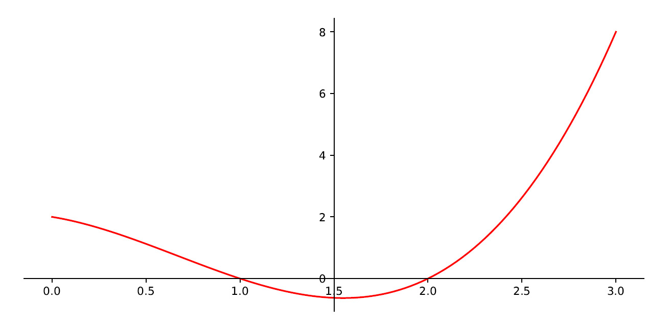
Figure 7.6 – The minimum point of the function

Here, we can see that the minimum of the function occurs for a value of x roughly equal to 1.5. This will be the value that we will have to determine through the gradient descent method. But to have the precise value so that we can compare it with what we will get later, we need to extract this value:

print('Value of x at the minimum of the function', x[np.argmin(y)])

To determine this value, we used numpy’s argmin() function. This function returns the position index of the minimum element in a vector. The following result is returned:

Value of x at the minimum of the function 1.5454545454545454

4. Now, let’s define the first and second derivative functions:

   FirstDerivative = lambda x: 3*x**2-4*x -1 

   SecondDerivative = lambda x: 6*x-4  
5. Now, we will initialize some parameters:

   actual_X  = 3 

   precision_value  = 0.000001 

   previous_step_size  = 1 

   max_iteration  = 10000 

   iteration_counter  = 0 

These parameters have the following meaning:

• The actual_X variable will contain the current value of the independent variable x. To start, we initialize it at x = 3, which represents the far-right value of the display range of the function in the graph.
• The precision_value variable will contain the value that defines the degree of precision of our algorithm. Being an iterative procedure, the solution is refined at each iteration and tends to converge. But this convergence may come after a very large number of iterations, so to save resources, it is advisable to stop the iterative procedure once adequate precision has been reached.
• The previous_step_size variable will contain the calculation of this precision and will be initialized to 1.
• The max_iteration variable contains the maximum number of iterations that we have provided for our algorithm. This value will be used to stop the procedure if it does not converge.
• Finally, the iteration_counter variable will be the iteration counter.

6. Now, we can apply the Newton-Raphson method, as follows:

   while previous_step_size  > precision_value  and iteration_counter  < max_iteration :

       PreviousX = actual_X 

       actual_X  = actual_X  - FirstDerivative(PreviousX)/ SecondDerivative(PreviousX)

       previous_step_size  = abs(actual_X  - PreviousX) 

       iteration_counter  = iteration_counter +1 

       print("Number of iterations = ",iteration_counter ,"
   Actual value of x  is = ",actual_X )

This procedure is similar to what we adopted to solve our problem in the Implementing gradient descent in Python section. A while loop, which will repeat itself until both conditions are verified (TRUE), was used here. When at least one of the two assumes a FALSE value, the cycle will be stopped. These two conditions provide a check on the precision and the number of iterations.

The Newton-Raphson method updates the current value of x, as follows:

At each step of the cycle, the previous value of x is stored in order to calculate the precision of the previous step as the absolute value of the difference between the two x values. In addition, the step counter is increased at each step. At the end of each step, the number of the iteration and the current value of x are printed, as follows:

Number of iterations =  1 
Actual value of x  is =  2.0
Number of iterations =  2 
Actual value of x  is =  1.625
Number of iterations =  3 
Actual value of x  is =  1.5516304347826086
Number of iterations =  4 
Actual value of x  is =  1.5485890147300967
Number of iterations =  5 
Actual value of x  is =  1.5485837703704566
Number of iterations =  6 
Actual value of x  is =  1.5485837703548635

As we mentioned in the Approaching Newton-Raphson for numerical optimization section, the number of iterations necessary to reach the solution is drastically skewed. In fact, we went from the 526 iterations necessary to bring the method based on the gradient’s descent to convergence to only 6 iterations for the Newton-Raphson method.

7. Finally, we will print the result:

   print("X value of f(x) minimum = ", actual_X )

The following result is returned:

X value of f(x) minimum =  1.5485837703548635

As we can verify, the returned value is very close to the exact value, which is equal to 1.5454545454545454. It differs precisely in terms of the value of the precision that we imposed as the term for the iterative procedure.

The secant method

A variant of Newton’s method is the secant method in which, at the step (n + 1), instead of considering the tangent to the curve of equation y = f (x) at the point of abscissa xn, the secant to the curve is constructed at the points of abscissa xn and xn − 1 respectively.

In other words, xn + 1 is calculated as the intersection of this secant with the abscissa axis. As with Newton’s method, the secant method also proceeds in an iterative way:

1. Given two initial values x0 and x1, x2 is calculated.
2. Then, with x1 and x2 known, x3 is calculated.

And so on.

Compared to Newton’s method, the secant method offers the advantage of not requiring the evaluation of the derivative of the function. Therefore, unlike the latter, it is also applicable when the function has no a priori known derivative. However, precisely in the vicinity of the solution, some computational problems may arise from the calculations.

Let’s now introduce stochastic gradient descent, an iterative method for the optimization of differentiable functions.

Deepening our knowledge of stochastic gradient descent

As we mentioned in the Exploring the gradient descent technique section, the implementation of the gradient descent method consists of initially evaluating both the function and its gradient, starting from a configuration chosen randomly in the space of dimensions.

From here, we try to move in the direction indicated by the gradient. This establishes a direction of descent in which the function tends to a minimum and examines whether the function actually takes on a value lower than that calculated in the previous configuration. If so, the procedure continues iteratively, recalculating the new gradient. This can be totally different from the previous one. After this, it starts again in search of a new minimum.

This iterative procedure requires that, at each step, the entire system status is updated. This means that all the parameters of the system must be recalculated. From a computational point of view, this equates to an extremely expensive operating cost and greatly slows down the estimation procedure. With respect to the standard gradient descent method, in which the weights are updated after calculating the gradient for the entire dataset, in the stochastic method, the system parameters are updated after a certain number of examples. These are chosen randomly in order to speed up the process and to try to avoid any local minimum situations.

Consider a dataset that contains n observations of a phenomenon. Here, let f be an objective function that we want to minimize with respect to a series of parameters x. Here, we can write the following equation:

From the analysis of the previous equation, we can deduce that the evaluation of the objective function f requires n evaluations of the function f, one for each value contained in the dataset.

In the classic gradient descent method, at each step, the function gradient is calculated in correspondence with all the values of the dataset through the following equation:

In some cases, the evaluation of the sum present in the previous equation can be particularly expensive, such as when the dataset is particularly large and there is no elementary expression for the objective function. The stochastic descent of the gradient solves this problem by introducing an approximation of the gradient function. At each step, instead of the sum of the gradients being evaluated in correspondence to the data contained in the dataset, the evaluation of the gradient is used only in a random subset of the dataset.

So, the previous equation replaces the following:

In the previous equation, 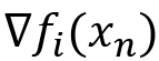is the gradient of one of the observations in the dataset, chosen randomly.

The pros of this technique are set out here:

• Based only on a part of the observations, the algorithm allows a wider exploration of the parametric space, with the greater possibility of finding new and potentially better points of the minimum
• Taking a step of the algorithm is computationally much faster, which ensures faster convergence toward the minimum point
• The parameter estimates can also be calculated by loading only a part of the dataset into memory at a time, allowing this method to be applied to large datasets

Now, let’s see how an iterative algorithm widely used to calculate maximum likelihood estimates works in the case of incomplete data.

Approaching the EM algorithm

The EM method is based on the notion of Maximum Likelihood Estimation (MLE) of θ, an unknown parameter of the data distribution. Given a sample space X, let x ∈ X be an observation extracted from the density f (x | θ), which depends on the parameter θ; we define the likelihood function of θ, given the single observation x in the following function:

The likelihood function is a conditional probability function, taken as a function of its second argument, keeping the first argument fixed.

When the sample consists of n independent observations, then the likelihood becomes this:

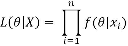
Since the values of the likelihood are very close to 0 and to simplify the calculation of the derivative for the maximum likelihood estimates of the parameters, it is appropriate to transform the function with a logarithmic transformation and therefore to study what is called log likelihood:

The goal of maximum MLE is to choose the parameters θ * that maximize the likelihood:

The EM algorithm is an iterative algorithm for MLE: the simplicity of the method is the reason why it has become very popular in the study of these types of problems. The idea of the algorithm alternates an Expectation phase, called E-step, which calculates the expected value of the log-likelihood of the parameter conditioned by the complete data and previous estimates of the parameter, and a maximization phase (Maximization), called M-step, which exploits the data just updated by the E-step to find the new estimated maximum likelihood value of the parameter. The procedure is repeated until the difference between the last iterations does not reach the predetermined tolerance threshold, demonstrating that the algorithm has reached convergence.

The E-step uses the elements of the mean vector and the covariance matrix to construct a set of regression equations that predict incomplete variable values from the observed variables. The purpose of this step is to predict the values of the parameters in a way that resembles the imputation of stochastic regression.

The next M-step applies the standard formulas for complete data to the newly created data to update the vector estimates of means and the variance and covariance matrix. The new parameter estimates are moved on to the next E-step, where a new set of regression equations are built to predict the unknown parameters again.

The EM algorithm repeats these two steps until the mean and the covariance matrix do not vary for several consecutive steps, and at that point, the algorithm converges to the MLEs. The concept behind EM is to use observable samples of latent variables to predict the values of samples that are not observable.

The EM algorithm offers the tools to solve a large number of problems; among these, we can list the following:

• Estimation of the values of latent variables
• Imputation of missing data in a dataset
• Estimation of the parameters of Finite Mixture Models (FMMs)
• Estimation of the parameters of Hidden Markov Models (HMMs)
• Unsupervised cluster learning

So, let’s see how to use EM to deal with Gaussian mixture problems.

EM algorithm for Gaussian mixture

The use of latent variables is a widely practiced solution for modeling complex distributions: properly selected, latent variables can greatly simplify the structure of the model. Latent variables are variables that are not directly observable and therefore not measurable, which therefore are hypothesized and analyzed through their effects. The links, the relationships, and the influences that a latent variable has on the other measurable variables become a way to go back to this hidden variable. Although larger, the joint distribution of observed and latent variables is often easier to manage than the marginal distribution of observed variables only. Models that make use of latent variables are referred to as latent variable models.

A popular class of latent variable models is mixed models: the methodology is based on dividing the responsibility of data modeling among several usually relatively simple components. The components are then combined using a blend distribution, giving each component a weight. Mixture models have several interesting properties: they can model arbitrary complex distributions while being easy to work with. For many common operations, the calculations can be performed independently for the individual components and for the distribution of the mixture. In addition, adapting the number of components provides an intuitive way to control the complexity of the model.

A mixture model is used as a probabilistic model to represent the presence of subpopulations within a population. It can also be defined as a mixed distribution that represents the probability distribution of some observations in the general population. Mixture models are used to create inferences, approximations, and predictions on the properties of subpopulations from observations or data acquired from the population under analysis.

Among the simple distributions, the Gaussian one is the most widely used. In the Normal distribution section of Chapter 3, Probability and Data Generation Processes, we defined this distribution. A normal distribution—also called a Gaussian distribution—has some important characteristics, is symmetrical and bell-shaped; its central position measures—the expected value and the median—coincide; its interquartile range is 1.33 times the mean square deviation; the random variable in a normal distribution takes values between -∞ and + ∞.

The goal of the Gaussian mixture model (GMM) is to find an approximation or estimate of its components, finding accommodation of the data that contains these components. It is not enough to explain the distributions of some data through a single statistical distribution if the data can be grouped into subpopulations or associated with different generation processes. It is necessary to use a composition of distributions, the same ones that are usually described by mixture models, which are defined by the parameters of each component and the proportions in which each of them contributes to the general distribution.

Gaussian mixtures are probabilistic models based on the assumption that the data belong to a mixture of different Gaussian distributions with unknown parameters. These models provide information on the center (mean) and on the variability (variance) of each cluster and provide the posterior probabilities. For example, if we have two distributions, if the data labels are known, we can go back to the parameters of the distributions (mean and variance); if the parameters are known, we can identify the labels. If, on the other hand, we do not have any information (parameters and labels), we can apply probabilistic algorithms to estimate the parameters.

The set of parameters that define these models can be estimated using many techniques: the EM algorithm is an iterative tool for estimating the maximum likelihood of mixed distributions. The principle of this tool is to introduce a multinomial indicator variable that identifies belonging to a specific cluster of each observation present in the dataset. In these models, the starting point is a random variable that is assumed to be extracted from a population that is an additive mixture of several subpopulations. The GMM generates a natural and intuitive representation of heterogeneity in a finite, usually small, number of latent classes, each considered as a type or group.

So, let’s see a practical application of the EM algorithm for estimating the parameters of a Gaussian mixture distribution. In this example, we will create two Gaussian distributions by setting the mean and standard deviation of each. Next, we will merge the newly generated data and try to estimate the parameters of this new distribution by modeling it as a Gaussian mixture. Our goal is to recover the parameters of the two starting Gaussian distributions.

As always, we will analyze the code line by line:

1. Let’s start by importing the libraries:

   import numpy as np

   import seaborn as sns

   from matplotlib import pyplot as plt

   from sklearn.mixture import GaussianMixture

   import pandas as pd

The numpy library is a Python library that contains numerous functions that can help us manage multidimensional matrices. Furthermore, it contains a large collection of high-level mathematical functions we can use on these matrices. Then, we imported the seaborn library, which is a Python library that enhances the data visualization tools of the matplotlib module. In the seaborn module, there are several features we can use to graphically represent our data. There are methods that facilitate the construction of statistical graphs with matplotlib. The matplotlib library is a Python library for printing high-quality graphics. Then, we imported the GaussianMixture() function from the sklearn.mixture module. This function estimates the parameters of a Gaussian mixture distribution using the EM algorithm. Finally, we imported the pandas library, which is an open source BSD-licensed library that contains data structures and operations to manipulate high-performance numeric values for the Python programming language.

2. Now, let’s set the Gaussian distribution parameters:

   mean_1=25

   st_1=9

   mean_2=50

   st_2=5

We then set the means and standard deviations of the two starting Gaussian distributions.

3. Now, let’s create two distributions:

   n_dist_1 = np.random.normal(loc=mean_1, scale=st_1, size=3000)

   n_dist_2 = np.random.normal(loc=mean_2, scale=st_2, size=7000)

To do this, we used the random.normal() function of the numpy library. Three parameters are passed: the mean, the standard deviation, and the number of samples to generate.

4. Now, we can merge the two distributions creating a single population:

   dist_merged = np.hstack((n_dist_1, n_dist_2))

The hstack() function of the numpy library stacks arrays in sequence horizontally (column-wise).

So, let’s see the population we created by drawing a histogram:

sns.set_style("white")
sns.histplot(data=dist_merged, kde=True)
plt.show()

We used the histplot() function of the seaborn library to return a univariate or bivariate histogram to show distributions of datasets. The following diagram is plotted:

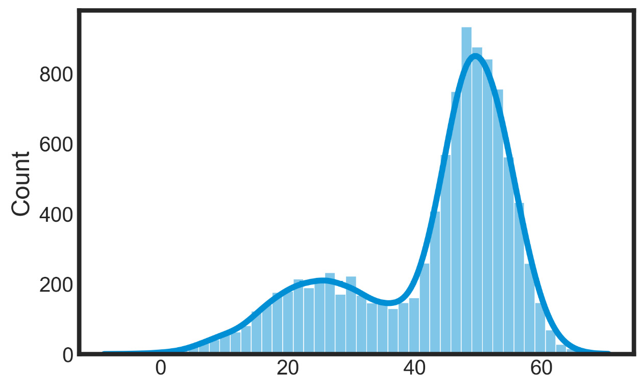
Figure 7.7 – Bivariate histograms of the datasets’ distributions

We can easily understand that the data contains two distributions—we just need to evaluate their parameters.

5. To do this, we will use the GMM:

   dist_merged_res = dist_merged.reshape((len(dist_merged), 1))

   gm_model = GaussianMixture(n_components=2, init_params='kmeans')

   gm_model.fit(dist_merged_res)

We first reshaped the population data into a format compatible with the GaussianMixture() function. K-means clustering is a partitioning method, and as anticipated, this method decomposes a dataset into a set of disjoint clusters. Given a dataset, a partitioning method constructs several partitions of this data, with each partition representing a cluster. These methods relocate instances by moving them from one cluster to another, starting from an initial partitioning. Finally, we applied the fit() function to fit the model using the merged initial Gaussian distribution.

6. Now, we can compare the parameters obtained from the simulation with the GMM with those of the initial distributions:

   print(f"Initial distribution means = {mean_1,mean_2}")

   print(f"Initial distribution standard deviation = {st_1,st_2}")

   print(f"GM_model distribution means = {gm_model.means_}")

   print(f"GM_model distribution standard deviation = {np.sqrt(gm_model.covariances_)}")

The following data is displayed:

Initial distribution means = (25, 50)
Initial distribution standard deviation = (9, 5)
GM_model distribution means = [[24.12193283]
                                    [49.87502388]]
GM_model distribution standard deviation = 
              [[[8.36021272]][[5.15620167]]]

Against initial means of 25 and 50, we obtained an estimate of 24.12 and 49.87—very close to the initial values. For the standard deviations, we estimated values equal to 8.3 and 5.15 compared to initial values equal to 9 and 5.

7. Using these parameters, we can now predict the class of each value of the distribution obtained by joining the two initial distributions:

   dist_labels = gm_model.predict(dist_merged_res)

In the previous line of code, we used the predict() function of the GMM. This function predicts the labels for the data samples in dist_merged_res using a trained model.

Let’s now see a representation of the distribution of the two classes:

sns.set_style("white")
data_pred=pd.DataFrame({'data':dist_merged, 'label':dist_labels})
sns.histplot(data = data_pred, x = "data", kde = True, hue = "label")
plt.show()

The following diagram is returned:

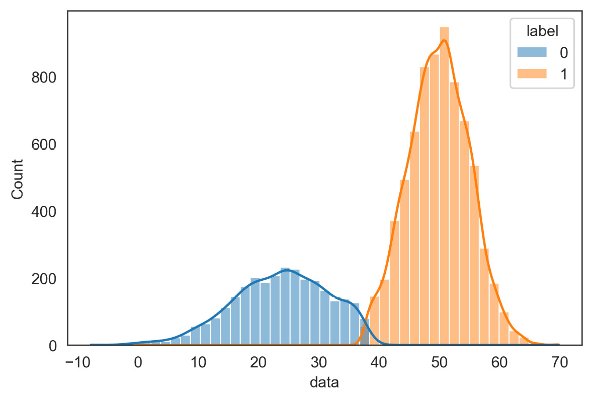
Figure 7.8 – Representation of the distribution of the two classes

8. To make a comparison between the initial distributions and those estimated with the GMM, we also represent the initial distributions:

   label_0 = np.zeros(3000, dtype=int)

   label_1 = np.ones(7000, dtype=int)

   labels_merged = np.hstack((label_1, label_0))

   data_init=pd.DataFrame({'data':dist_merged, 'label':labels_merged})

We first created two vectors containing the labels of the two classes with the same number of elements as the initial distributions. We then stacked them in a single vector and created a pandas DataFrame of two columns: in the first, we inserted the merged distribution, while in the second column, we added the labels.

All that’s required is to display the result:

sns.set_style("white")
sns.histplot(data = data_init, x = "data", kde = True, hue = "label")
plt.show()

The following diagram is displayed:

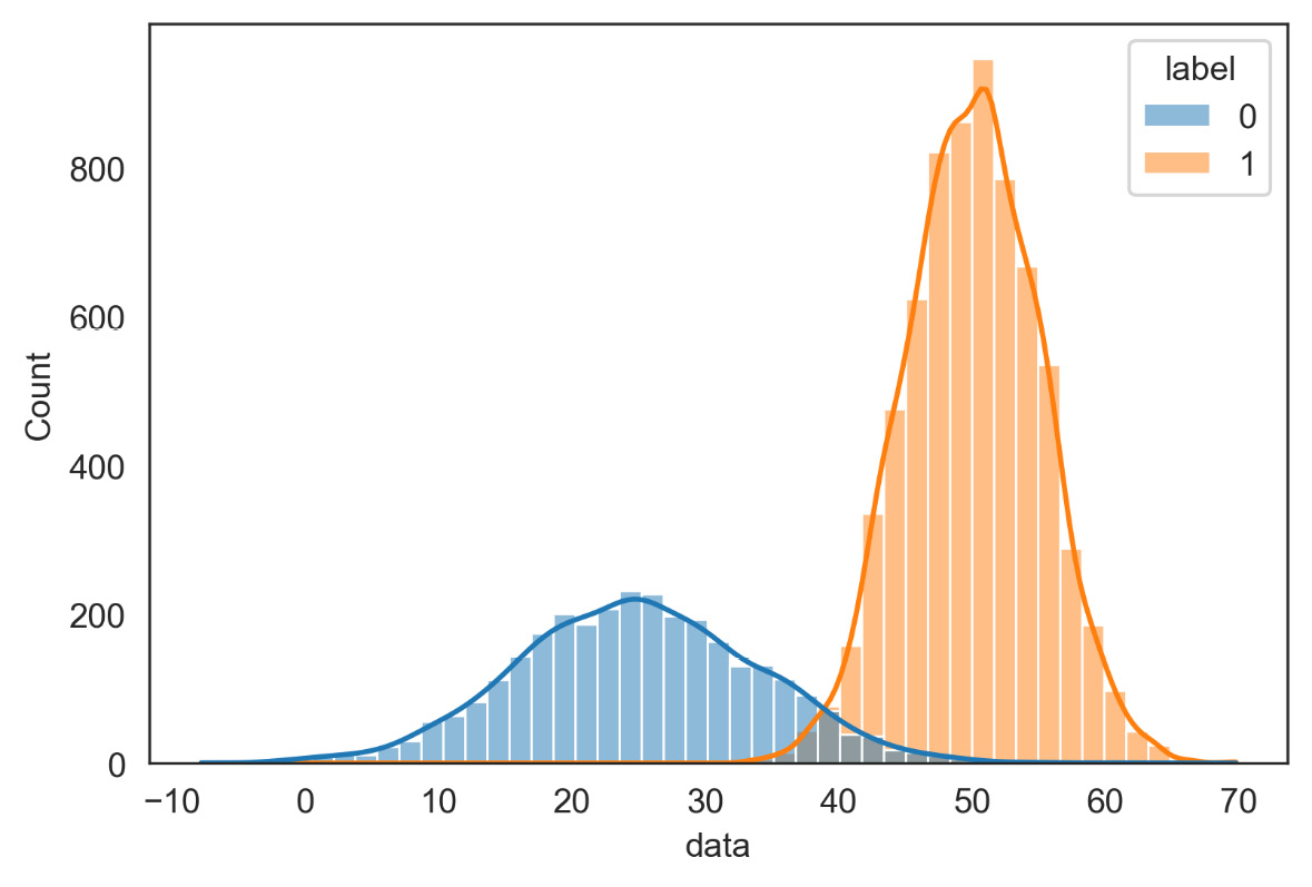
Figure 7.9 – Initial distributions of the two classes

From the comparison of Figures 7.8 and 7.9, we can appreciate the quality of the estimate of the parameters of the two distributions: it should be noted that this estimate was carried out without knowing any information on the starting distributions.

After analyzing in detail, a practical case of application of the EM method, we will now study another optimization method.

Understanding Simulated Annealing (SA)

The SA algorithm is a general optimization technique for solving combinatorial optimization problems. The algorithm is based on stochastic techniques and iterative improvement algorithms.

Iterative improvement algorithms

Search algorithms and iterative improvement of solutions are known as local search algorithms. The operation of these algorithms involves the following steps:

1. Starting from configuration A, a sequence of iterations is performed, each of which consists of a transition from the current configuration to another that belongs to the neighborhood of A.
2. If the transition gives rise to an improvement of the cost function, the current configuration is replaced by its neighbor; otherwise, a new configuration among the neighboring ones is selected for a new comparison.
3. The algorithm ends when a configuration is obtained that has a cost no worse than any other neighboring configuration.

This class of algorithms has some disadvantages:

• By definition, the local search algorithm ends in a local minimum, and there is no information on how much this minimum differs from the global minimum
• The quality of the obtained local minimum depends on the initial configuration chosen and no general criterion establishes a way to select a starting point from which to obtain good solutions
• In general, no limits can be given to the completion time of the algorithm

However, the local search has the advantage of being generally applicable with ease: the definition of the configurations, the cost function, and the generation mechanism do not generally create problems.

To remedy the aforementioned disadvantages, some variations have been introduced in the algorithm:

• Execution of the algorithm on a high number of initial configurations uniformly distributed over the set of possible configurations
• Use of the information obtained from the previous executions to improve the choice of the initial configuration for the subsequent computation
• Introduction of a more complex generation mechanism to make the algorithm capable of surpassing the local optimum

In addition, configurations are accepted that provide a worsening of the value from the cost function; in general, however, the local search algorithm accepts only improvements in the cost of the solutions. This variant of improvement is provided for by the SA algorithm: the solutions obtained with the approximation algorithm based on the SA algorithm do not depend on the initial configuration and are generally able to approximate the overall optimum well. SA finds the global optimum asymptotically, does not show the disadvantages of the local search algorithm, and is equally an algorithm applicable to the generality of problems.

SA in action

The SA algorithm is based on the analogy between the solidification process of metals and the problem of solving complex combinatorial problems. In physics, the term annealing denotes a physical process in which a solid is progressively heated up to a temperature at which it reaches the liquid state, and then slowly cooled. In this way, if the temperature reached is high enough and the cooling process is slow enough, all the molecules are arranged in a configuration of minimum energy.

During this phase, changes of state occur in the direction of decreasing energies: transitions from an i state to a j state of the solid involving energy increases can still occur with a probability defined by the following equation:

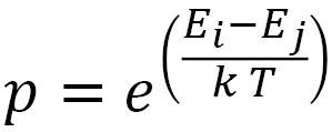
In the previous equation:

• are the energies associated with the two states
• k is Boltzmann’s constant
• T is the temperature of the metal

This model is exploited in SA to solve optimization problems. In this case, an analogy is proposed between the objective function of the problem and energy, while the temperature becomes the control variable of the algorithm. During the search for the optimal solution, therefore, in addition to solutions that lead to improvements in the objective function, those that lead to worsening are also accepted, with a temperature-dependent acceptance probability according to the previous equation. This feature translates into the main advantage of SA, which is the ability to expand the search space for solutions and overcome the local minima of the objective function.

The SA algorithm foresees the following steps: initially, a high value is given to the control parameter; then, a sequence of configurations is generated, up to the minimum point of the objective function. The configurations are chosen among those present in the neighborhood of the current solution, according to the following criterion: if the difference between the values of the objective function <0, then the new configuration replaces the old one; otherwise, if the difference between the values of the objective function ≥ 0, the probability of replacing the old configuration with the new one is calculated according to the previous equation. So, there is a non-negative probability of accepting solutions with higher objective functions. The process continues until the probability distribution of the configurations approaches the Boltzmann distribution.

The value of the control parameter is progressively lowered in discrete steps, and the system is allowed to reach equilibrium at each step. In the initial part of the algorithm, when the temperature value is high, the acceptability criterion will also be high: in this first phase, it will therefore be possible to examine many permutations and then explore the entire search domain. As the temperature drops and the model approaches its minimum energy state, only the smallest energy deviations are accepted: this is reminiscent of gradient descent as it only considers the local search space and focuses only on improving the solution.

The temperature parameter plays an essential role in finding the global optimum of an optimization problem: it is set to regulate the slow decrease in the probability of accepting worse solutions while the entire solution space is explored.

The algorithm ends with a control value, beyond which no configuration that worsens the value of the objective function is accepted. The solution thus obtained is the solution to the problem treated. The method, therefore, leverages a global optimizer that explores the search space early on and a local optimizer that leverages only what is critical to achieving good results. It should be noted that this method does not protect us from possible stagnation in a position of local minimum. The method is very sensitive to parameter values, which makes tuning difficult: parameter adjustment difficulty is the greatest weakness of SA.

So, let’s see a practical application of this algorithm (simulated_annealing.py). As always, we will analyze the code line by line:

1. Let’s start by importing the necessary libraries:

   import numpy as np

   import matplotlib.pyplot as plt

We first imported the numpy library, which is a Python library that contains numerous functions that can help us manage multidimensional matrices. Furthermore, it contains a large collection of high-level mathematical functions we can use on these matrices. Then, we imported the matplotlib library, a Python library for printing high-quality graphics.

2. Let’s now create an exploration domain and a function we want to minimize:

   x= np.linspace(0,10,1000)

   def cost_function(x):

       return x*np.sin(2.1*x+1)

We first created an array of 1000 elements equally spaced between the extreme values 0 and 10. This represents the domain of existence of our function—that is, the space in which we are going to look for the solution. Next, we created a sinusoidal function that represents our objective function; the form of the function was chosen because it has different minima. To confirm this, let’s see a representation of it:

plt.plot(x,cost_function(x))
plt.xlabel('X')
plt.ylabel('Cost Function')
plt.show()

The following diagram is displayed:

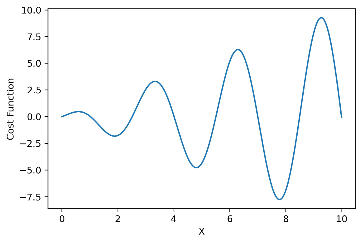
Figure 7.10 – Cost function representation

In this way, we confirm the presence of three lows in the 0-10 range.

3. Now, let’s fix the parameters of the method:

   temp = 2000

   iter = 2000

   step_size = 0.1
4. Now, let’s move on to initializing the system variables:

   np.random.seed(15)

   xi = np.random.uniform(min(x), max(x))

   E_xi = cost_function(xi)

   xit, E_xit = xi, E_xi

   cost_func_eval = []

   acc_prob = 1

To start, we set the seed of the random number generation using the np.random.seed() numpy function: this function initializes the basic random number generator. Next, we set the first value of x in which to evaluate the cost function. To do this, we used the random.uniform() numpy function: this function generates numbers within a defined numeric range. In this case, the range is between the extreme values of the x variable setting range. Next, we made an evaluation of the cost function for that value of x. After doing this, we initialized some temporary variables that we will need in the iterative procedure. Our aim is to set a temporary x variable, evaluate the cost function, and check if this value is acceptable. Acceptable values are stored in an array created ad hoc (cost_func_eval). Finally, we initialized the acc_prob variable, which will contain the acceptance probability.

5. Now, we can start the iterative procedure:

   for i in range(iter):

           xstep = xit + np.random.randn() * step_size  

           E_step = cost_function(xstep)

At each cycle, we set a value for x by adding to the previous value a term obtained by multiplying the step size by a random number. In correspondence with this new value of x, we then carry out an evaluation of the function.

We can therefore carry out our first check:

        if E_step < E_xi:
            xi, E_xi = xstep, E_step
            cost_func_eval.append(E_xi)
            print('Iteration = ',i, 
               'x_min = ',xi,'Global Minimum =', E_xi,
               'Acceptance Probability =', acc_prob)

If the estimated energy is less than what has been accepted so far, then we update the improvement values. This value is first added to the cost_func_eval array, and the information on the improvement obtained is printed on the screen:

        diff_energy = E_step - E_xit
        t = temp /(i + 1)
        acc_prob = np.exp(-diff_energy/ t)

In this block of code, we evaluate the acceptance probability according to what is indicated in the equation seen at the beginning of this section. We first evaluate the difference between the energies, then update the temperature value, and finally evaluate the acceptance probability.

Finally, we decide whether to accept the new point:

        if diff_energy < 0 or 
                np.random.randn() < acc_prob:
            xit, E_xit = xstep, E_step

In conclusion, we draw a graph with the cost function improvement procedure during the iterative procedure:

plt.plot(cost_func_eval, 'bs--')
plt.xlabel('Improvement Step')
plt.ylabel('Cost Function improvement')
plt.show()

The following diagram is displayed:

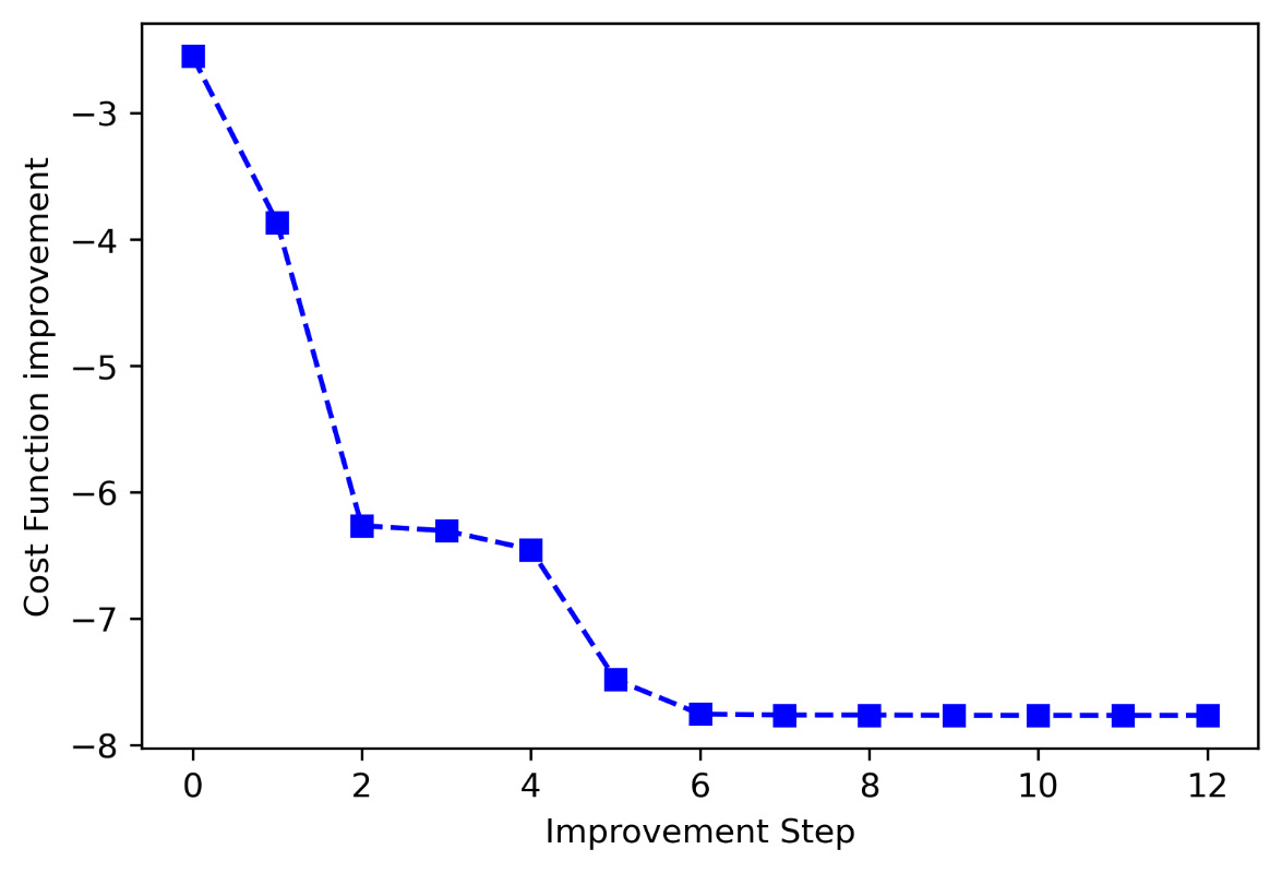
Figure 7.11 – Cost function improvement

To conclude, we report an extract of the information regarding some accepted improvement steps:

Iteration =  0 x_min =  8.352060345432603 Global Minimum = -2.549691087509061 Acceptance Probability = 1
Iteration =  1 x_min =  8.268146731695177 Global Minimum = -3.865265080181498 Acceptance Probability = 1.0011720530797679
Iteration =  2 x_min =  8.077074224781931 Global Minimum = -6.264757086553908 Acceptance Probability = 1.0013164397397474
Iteration =  4 x_min =  8.072960126990173 Global Minimum = -6.3053561226675905 Acceptance Probability = 0.9993874938212183
Iteration =  14 x_min =  8.057426141282635 Global Minimum = -6.45398523520768 Acceptance Probability = 1.0011249991583007
Iteration =  17 x_min =  7.908942504770391 Global Minimum = -7.482144101692382 Acceptance Probability = 0.9960707945643333
Iteration =  18 x_min =  7.805571271239743 Global Minimum = -7.755842336539771 Acceptance Probability = 1.0092963751415767
Iteration =  21 x_min =  7.767739570791674 Global Minimum = -7.763382995462104 Acceptance Probability = 1.0072493114830527
Iteration =  27 x_min =  7.793961859355448 Global Minimum = -7.763418087146118 Acceptance Probability = 0.9975392161808777
Iteration =  36 x_min =  7.775446728598834 Global Minimum = -7.765853968129766 Acceptance Probability = 1.007367947545534
Iteration =  41 x_min =  7.778624797903834 Global Minimum = -7.766277157406623 Acceptance Probability = 0.9981491502724658
Iteration =  138 x_min =  7.781197205345049 Global Minimum = -7.766364644616736 Acceptance Probability = 1.036566292077183
Iteration =  1174 x_min =  7.78075358444397 Global Minimum = -7.7663658475723265 Acceptance Probability = 1.3178155041756248

From the comparison between the graph of the trend of the cost function and the final value obtained, we can conclude that the algorithm has brought us in correspondence with the global minimum.

After analyzing some optimization procedures with practical examples, let’s now see other multivariate optimization methods available in the SciPy library.

Discovering multivariate optimization methods in Python

In this section, we will analyze some numerical optimization methods contained in the Python SciPy library. SciPy is a collection of mathematical algorithms and functions based on numpy. It contains a series of commands and high-level classes that can be used to manipulate and display data. With SciPy, functionality is added to Python, making it a data processing and system prototyping environment, similar to commercial systems such as MATLAB.

Scientific applications that use SciPy benefit from the development of add-on modules in numerous fields of numerical computing made by developers around the world. Numerical optimization problems are also covered among the available modules.

The SciPy optimize module contains numerous functions for the minimization/maximization of objective functions, both constrained and unconstrained. It treats nonlinear problems with support for both local and global optimization algorithms. In addition, problems regarding linear programming, constrained and nonlinear least squares, search for roots, and the adaptation of curves are treated. In the following sections, we will analyze some of them.

The Nelder-Mead method

Most of the well-known optimization algorithms are based on the concept of derivatives and on the information that can be deduced from the gradient. However, many optimization problems deriving from real applications are characterized by the fact that the analytical expression of the objective function is not known, which makes it impossible to calculate its derivatives, or because is particularly complex, so coding the derivatives may take too long. To solve this type of problem, several algorithms have been developed that do not attempt to approximate the gradient but rather use the values of the function in a set of sampling points to determine a new iteration by other means.

The Nelder-Mead method tries to minimize a nonlinear function by evaluating test points that constitute a geometric form called a simplex.

Important note

A simplex is defined as a set of closed and convex points of a Euclidean space that allow us to find the solution to the typical optimization problem of linear programming.

The choice of geometric figure for the simplex is mainly due to two reasons: the ability of the simplex to adapt its shape to the trend in the space of the objective function deforming itself, and the fact that it requires the memorization of only n + 1 points. Each iteration of a direct search method based on the simplex begins with a simplex, specified by its n + 1 vertices and the values of the associated functions. One or more test points and the respective values of the function are calculated, and the iteration ends with a new simplex so that the values of the function in its vertices satisfy some form of descent condition with respect to the previous simplex.

The Nelder-Mead algorithm is particularly sparing in terms of its evaluation of the function at each iteration, given that, in practice, it typically requires only one or two evaluations of the function to build a new simplex. However, since it does not use any gradient assessment, it may take longer to find the minimum.

This method is easily implemented in Python using the minimize routine of the SciPy optimize module. Let’s look at a simple example of using this method:

1. Let’s start by loading the necessary libraries:

   import numpy as np

   from scipy.optimize import minimize

   import matplotlib.pyplot as plt

   from matplotlib import cm

   from matplotlib.ticker import LinearLocator, FormatStrFormatter

   from mpl_toolkits.mplot3d import Axes3D

The library that’s needed to generate 3D graphics is imported (Axes3D).

2. Now, let’s define the function:

   def matyas(x):

      return 0.26*(x[0]**2+x[1]**2)-0.48*x[0]*x[1]

The matyas function is continuous, convex, unimodal, differentiable, and non-separable, and is defined on two-dimensional space. The matyas function is defined as follows:

This function is defined on a x,y [-10,10]. This function has one global minimum in f(0,0) = 0.

3. Let’s visualize the matyas function:

   x = np.linspace(-10,10,100)

   y = np.linspace(-10,10,100)

   x, y = np.meshgrid(x, y)

   z = matyas([x,y])

   fig = plt.figure()

   ax = fig.gca(projection='3d')

   surf = ax.plot_surface(x, y, z, rstride=1, cstride=1, 

                         cmap=cm.RdBu,linewidth=0, antialiased=False)

   ax.zaxis.set_major_locator(LinearLocator(10))

   ax.zaxis.set_major_formatter(FormatStrFormatter('%.02f'))

   fig.colorbar(surf, shrink=0.5, aspect=10)

   plt.show()

To start, we defined independent variables, x and y, in the range that we have already specified [-10.10]. So, we created a grid using the numpy meshgrid() function. This function creates an array in which the rows and columns correspond to the values of x and y. We will use this matrix to plot the corresponding points of the z variable, which corresponds to the matyas function. After defining the x, y, and z variables, we traced a three-dimensional graph to represent the function. The following diagram is plotted:

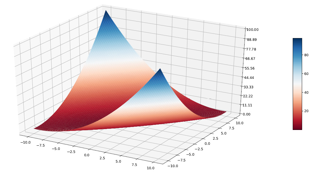
Figure 7.12 – Meshgrid plot to represent the function

4. As we already mentioned, the Nelder-Mead method does not require us to calculate a derivative as it is limited to evaluating the function. This means that we can directly apply the method, like so:

   x0 = np.array([-10, 10])

   NelderMeadOptimizeResults = minimize(matyas, x0,

               method='nelder-mead',

               options={'xatol': 1e-8, 'disp': True})

   print(NelderMeadOptimizeResults.x)

To do this, we first defined an initial point to start the search procedure from for the minimum of the function. So, we used the minimize() function of the SciPy optimize module. This function finds the minimum of the scalar functions of one or more variables. The following parameters have been passed:

• matyas: The function you want to minimize
• x0: The initial vector
• method = 'nelder-mead': The method used for the minimization procedure

Additionally, the following two options have been added:

• 'xatol': 1e-8: Defines the absolute error acceptable for convergence
• 'disp': True: Set to True to print convergence messages

5. Finally, we printed the results of the optimization method, as follows:

   Optimization terminated successfully.

            Current function value: 0.000000

            Iterations: 77

            Function evaluations: 147

   [3.17941614e-09 3.64600127e-09]

The minimum was identified in the value 0, as already anticipated. Furthermore, this value was identified in correspondence with the following values:

X = 3.17941614e-09 
Y = 3.64600127e-09

These are values that are very close to zero, as we expected. The deviation from this value is consistent with the error that we set for the method.

Powell’s conjugate direction algorithm

Conjugate direction methods were originally introduced as iterative methods for solving linear systems with a symmetric and positive definite coefficient matrix, and for minimizing strictly convex quadratic functions.

The main feature of conjugated direction methods for minimizing quadratic functions is that of generating, in a simple way, a set of directions that, in addition to being linearly independent, enjoy the further important property of being mutually conjugated.

The idea of Powell’s method is that if the minimum of a quadratic function is found along each of the p (p <n) directions in a stage of the research, then when taking a step along each direction, the final displacement from the beginning up to the p-th step is conjugated with respect to all the p subdirections of research.

For example, if points 1 and 2 are obtained from one-dimensional searches in the same direction but from different starting points, then the line formed by 1 and 2 will be directed toward the maximum. The directions represented by these lines are called conjugate directions.

Let’s analyze a practical case of applying the Powell method. We will use the matyas function, which we defined in the The Nelder-Mead method section:

1. Let’s start by loading the necessary libraries:

   import numpy as np

   from scipy.optimize import minimize
2. Now, let’s define the function:

   def matyas (x):

       return 0.26 * (x [0] ** 2 + x [1] ** 2) -0.48 * x [0] * x [1]
3. Now, let’s apply the method:

   x0 = np.array([-10, 10])

   PowellOptimizeResults = minimize(matyas, x0, 

              method='Powell',

              options={'xtol': 1e-8, 'disp': True})

   print(PowellOptimizeResults.x)

The minimize() function of the SciPy optimize module was used here. This function finds the minimum of the scalar functions of one or more variables. The following parameters were passed:

• matyas: The function we want to minimize
• x0: The initial vector
• method = 'Powell': The method used for the minimization procedure

Additionally, the following two options have been added:

• 'xtol': 1e-8: Defines the absolute error acceptable for convergence
• 'disp': True: Set to True to print convergence messages

4. Finally, we printed the results of the optimization method. The following results are returned:

   Optimization terminated successfully.

           Current function value: 0.000000

           Iterations: 3

           Function evaluations: 66

   [-6.66133815e-14 -1.32338585e-13]

The minimum was identified in the value 0, as specified in the The Nelder-Mead method section. Furthermore, this value was identified in correspondence with the following values:

X = -6.66133815e-14
Y = -1.32338585e-13

These are values very close to zero, as we expected. We can now make a comparison between the two methods we applied to the same function. We can note that the number of iterations necessary to reach convergence is equal to 3 for the Powell method, while it is equal to 77 for the Nelder-Mead method. A drastic reduction in the number of evaluations of the function is also noted: 66 against 147. Finally, the difference between the calculated value and the expected value is reduced by the Powell method.

Summarizing other optimization methodologies

The minimize() routine of the SciPy optimize package contains numerous methods for unconstrained and constrained minimization. We analyzed some of them in detail in the previous sections. In the following list, we have summarized the most used methods provided by the package:

• Newton-Broyden-Fletcher-Goldfarb-Shanno (BFGS): This is an iterative unconstrained optimization method used to solve nonlinear problems. This method looks for the points where the first derivative is zero.
• Conjugate Gradient (CG): This method belongs to the family of conjugate gradient algorithms and performs a minimization of the scalar function of one or more variables. This method requires that the system matrix be symmetric and positive definite.
• dog-leg trust-region (dogleg): The method first defines a region around the current best solution, where the original objective function can be approximated. The algorithm thus takes a step forward within the region.
• Newton-CG: This method is also called truncated Newton’s method. It is a method that identifies the direction of research by adopting a procedure based on the conjugate gradient, to roughly minimize the quadratic function.
• Limited-memory BFGS (L-BFGS): This is part of the family of quasi-Newton methods. It uses the BFGS method for systematically saving computer memory.
• Constrained Optimization By Linear Approximation (COBYLA): The operating mechanism is iterative and uses the principles of linear programming to refine the solution found in the previous step. Convergence is achieved by progressively reducing the pace.

Summary

In this chapter, we learned how to use different numerical optimization techniques to improve the solutions offered by a simulation model. We started by introducing the basic concepts of numerical optimization, defining a minimization problem, and learning to distinguish between local and global minimums. We then moved on and looked at the optimization techniques based on gradient descent. We defined the mathematical formulation of the technique and gave it a geometric representation. Furthermore, we deepened our knowledge of the concepts surrounding the learning rate and trial and error. By doing this, we addressed a practical case to reinforce the concepts we learned by solving the problem of searching for the minimum of a quadratic function.

Subsequently, we learned how to use the Newton-Raphson method to search for the roots of a function and then how to exploit the same methodology for numerical optimization. We also analyzed a practical case for this technology to immediately put the concepts we learned into practice. We did this by looking for the local minimum of a convex function.

We then went on to study the stochastic gradient descent algorithm, which allows us to considerably reduce the computational costs of a numerical optimization problem. This result is obtained by using a single estimate of the gradient at each step, which is chosen in a stochastic way among those available. Then, we analyzed the EM algorithm and the SA method to improve the optimization procedure.

Finally, we explored the multivariate numerical optimization algorithms contained in the Python SciPy package. For some of them, we defined the mathematical formulation and proposed a practical example of using the method. For the others, a summary was drawn up to list their characteristics.

In the next chapter, we will learn the basic concepts of soft computing and how to implement genetic programming. We will also understand genetic algorithm techniques, and we will learn how to implement symbolic regression and how to use the Cellular Automation (CA) model.