Chapter 3. The Wrong Way to Draw a Line

If there is one thing computers excel at, it’s following instructions with a high degree of accuracy. This is partly why they have revolutionized design, architecture, manufacturing, the sciences, and countless other fields.

But precision is of only limited interest to us in the context of generative art. There is a certain joylessness in perfect accuracy; the natural world isn’t like that. If our art were to achieve such perfection, it might be dismissed as overly mechanical.

Obversely, although we may crave forms with imperfection and unpredictability, we don’t want that imperfection to wander too far into indistinction, either. We’re looking for the sweet spot: that balance between the organic and the mechanical, between chaos and order. To find this, we may need to move away from the efficient, programmatic way of drawing lines and nudge the process toward something a little less deterministic.

In this chapter (and the next), I’ll explain and demonstrate a core principle behind my particular approach to programmatic art: breaking down even the simplest of processes, and allowing a touch of chaos to creep in. The “right” way to draw a line, according to a machine, is always the most efficient and accurate way of getting from point A to point B. But from an artistic standpoint, it’s the “wrong” way that is the often the most interesting.

3.1. Randomness and not-so-randomness

It may be argued that all generative art has to include a degree of randomness; without randomness, there can be no unpredictability, can there? This isn’t strictly true. A call to a random-number-generating function isn’t always necessary in order to come up with something that appears unpredictable to our limited human calculating faculties. Mathematical formulae above a certain degree of sophistication always return predictable results, yes, but the result may only be predictable to another calculating device of comparable sophistication. It may be beyond what a human observer can project.

Almost all programming languages include a function equivalent to Processing’s random function, but returning a truly random number is an impossibility for a predictable machine. Computer-generated randomness is always pseudo-random, using mathematical formulae, often including a reference to the machine’s internal clock as one of its factors to ensure that no two calculations give the same result. The formulae behind these functions are an art in themselves, but you need only trust that a returned random value will be good enough to fool us dumb humans.

I may make light of the topic, but pseudo-randomness is a significant problem in computer science, mainly because of its use in data encryption. If you want to get really anally retentive about your randomness, you’ll love the random.org project run by Dublin Trinity College’s School of Computer Science. It has an online API for returning “true” random numbers based on atmospheric noise. But this only moves the debate into the realm of chaos math and the questionable quantum predictability or unpredictability of the natural world.

Using random is simple. A random function typically returns a value in the range 0 to 1, which you can then manipulate to give a value within any given range. In Processing, you pass a parameter to give a maximum value, or two parameters to return a number within a range. For example, if you want a number in the range 20 to 480, you can use

float randnum = random(460) + 20;

Or you can also write it like this:

float randnum = random(20, 480);

I prefer the first notation, even though the range is less obvious upon reading. Later in this chapter, you’ll use functions that can only return values between 0 and 1; you won’t have the convenience of passing a range to them, which is why I force myself to get used to thinking of variance without Processing’s more convenient convention. Without using any parameters, you can express any random range as follows:

float randnum = (random(1) * (max+min)) – min;

Let’s apply this to the drawing of a line. If a line is what you’re after, there is an easy way to connect point A to point B (see figure 3.1):

Figure 3.1. The correct way to draw a line

size(500,100);
background(255);
strokeWeight(5);
smooth();

stroke(20, 50, 70);
line(20,50,480,50);

Randomizing the line is then just a matter of replacing the parameters. Note how you use the width and height constants, even though you know the width is 500 and the height is 100. It means the script will adapt to these relative values if you decide to change width or height later. Even if you have no intention of doing such a thing, it’s a good habit to get into:

stroke(0, 30);
line(20,50,480,50);

stroke(20, 50, 70);
float randx = random(width);
float randy = random(height);
line(20,50,randx, randy);

Figure 3.2 shows a possible output. Without wanting to be too judgmental of your first piece of generative drawing, this is rather uninteresting. It’s just not doing it for me I’m afraid. Still the line is too controlled, too tightly gripped by the machine’s way of drawing. To overcome this, we need to take a step back from the language’s useful conveniences and deconstruct it a little.

Figure 3.2. A rather uninteresting random line

3.2. Iterative variance

We know the computer is capable of getting from point A to B with maximum efficiency, but efficiency isn’t necessarily useful aesthetically. To make things more interesting, we need to take a step back from the “best” way of drawing a line and look at some less optimal options. You could start by breaking the line-drawing process into a series of steps.

The following code chunk uses a for loop to iterate through the x position in 10-pixel steps, keeping track of the last x and y positions so it can draw a micro-line back to the previous point. The line is constructed as a chain of 46 links. The resulting image in the output window will look exactly the same as that shown in figure 3.1: a line from point 20,50 to 480,20. But you’re now using a few more lines of code:

int step = 10;
float lastx = -999;
float lasty = -999;
float y = 50;
int border = 20;
for (int x=border; x<=width-border; x+=step) {
 if (lastx > -999) {
    line(x, y, lastx, lasty);
  }
  lastx = x;
  lasty = y;
 }

If this were an old lady you were helping across the road, and you insisted on instructing her every footstep—“Now move your left foot a few centimeters, then your right ...”—she’d probably think you were crazy, and be checking her purse. But it’s impossible to patronize a computer program. Believe me, I’ve tried. Pointless, tedious, and seemingly arbitrary instructions are perfectly fine and won’t be criticized. Our machines are capable of carrying out dumb instructions as smoothly and efficiently as they would execute “good” code.

This staccato drawing style enables you to start adding a more interesting flavor of randomness to your line. Add an instruction to vary the y value with every step:

int step = 10;
float lastx = -999;
float lasty = -999;
float y = 50;
int borderx=20;
int bordery=10;
for (int x=borderx; x<=width-borderx; x+=step) {
 y = bordery + random(height - 2*bordery);
 if (lastx > -999) {
    line(x, y, lastx, lasty);
  }
  lastx = x;
  lasty = y;
}

The first line in the loop assigns y a random value between 10 and 90. The result is shown in figure 3.3.

Figure 3.3. Introducing randomness to the y position

How easily the line develops an unpredictability. The line will be different every time you run the script. But perhaps you’ve wandered too far in the direction of chaos. Let’s pull back on the randomness reins a little. In the following example, instead of just making the y position random in a range, you add or subtract a random amount from the previous y value, creating a more natural variance:

float xstep = 10;
float ystep = 10;
float lastx = 20;
float lasty = 50;
float y = 50;
for (int x=20; x<=480; x+=xstep) {
 ystep = random(20) - 10;  //range -10 to 10
 y += ystep;
  line(x, y, lastx, lasty);
  lastx = x;
  lasty = y; }

The result is shown in figure 3.4.

Figure 3.4. Random variance looks better than plain randomness.

This is starting to look better. Yes, a raggedy line is what I’m calling “better” in this context: the line is less controlled, yet not so chaotic as to be useless.

You’ve drawn only a single line so far, but already you can see a touch of the analogue creeping into the output. You can refine this further to get a gentler progression, or dive in and start drawing more shapes using this method; but first I want to show you a much easier way of giving your lines naturalistic forms. Wherever you can use random, you can use noise, which is what you’ll play with next.

3.3. Naturalistic variance

There aren’t many programming awards that your mom has heard of. So on the day Ken Perlin bought home an Oscar—an Academy of Motion Picture Arts and Sciences award—for an algorithm he created, I’d imagine it was a rare case of a programmer’s mother phoning all her friends and praising his decision to devote his life to communing with the calculating machines.

The Technical Achievement Oscar that Ken was (rather belatedly) awarded in 1997 was for his work on procedural textures developed while working on the graphics for the science fiction film TRON (1982). TRON was a pioneering movie in both subject matter and production. It made a hero of a video gamer at a time when video games were seen as an idiotic frivolity; and much of the film took place in virtual reality, two years before William Gibson’s Neuromancer was credited with popularizing the concept of cyberspace. Most significantly, though, it was one of the first films to rely heavily on computer graphics for its special effects.

Ken’s job was to develop textures to give 3D objects a more natural appearance. He was looking for ways to generate randomness in a controlled fashion, much like we were in the previous section. The function he came up with to do this, his Perlin noise, is really just another pseudorandom function—but it’s a bloody good one, one specifically attuned to natural-looking visuals. If you’re interested in the logic behind it, you can view the code, along with examples of Ken’s applications of it, on his website: http://mrl.nyu.edu/~perlin/.

By the late 1980s, Ken Perlin’s noise functions were pretty much ubiquitous. It’s probably safe to say that if you’ve ever played a graphical console game, or seen a computer-animated film, or seen CGI used in any movie made in the last 20 years, you’ve seen Ken’s work in action. Now, with Processing, Ken’s algorithms are encapsulated into a simple function—noise—that enables you to harness in your own creations the same naturalistic variance seen on the big screen.

3.3.1. Perlin noise in Processing

noise is generally used to produce a sequence of numbers. You pass it a series of seed values, each of which returns a noise value between 0 and 1 calculated according to the values that precede and follow it. It doesn’t matter where you start the sequence of values, but it’s a good idea to randomize the start point; otherwise, the resulting line will be identical every time. Small increments, between 0 and 0.1, usually give the best results.

Probably the best way to get an appreciation of noise is to try using it. Listing 3.1 takes the script from the last section and replaces the call to random with a noise sequence.

Listing 3.1. Perlin noise

In this example, the sequence of values starts somewhere between 0 and 10 (random(10)) and increments by 0.1 every step of the loop. The call to noise() for every seed value in the sequence returns a floating-point number between 0 and 1, which you adapt (multiply by 80, add 10) to produce a useful y value between 10 and 90. The result (one possible result, anyway) is shown in figure 3.5.

Figure 3.5. Perlin noise: a possible output of listing 3.1

For a smoother result, you can reduce the x step to 1, so the line steps only one pixel at a time horizontally; reduce the ynoise step accordingly. Figure 3.6 shows a single-pixel x step with ynoise steps of 0.03.

Figure 3.6. Perlin noise, with ynoise increment of 0.03 for every x pixel

It’s a handy trick. But don’t think Ken Perlin is the only person who can write an interesting variance function.

3.3.2. Creating your own noise

As mentioned at the start of this chapter, when you call a function such as noise or random, you aren’t plucking a value from the ether; the function returns the result of a calculation. The calculation may be deliberately abstract, as in the case of random—so abstract as to appear utterly unpredictable (although, obviously, it is predictable if you know the formula), but it’s still just a calculation. I don’t want you to think these are the only calculations you can use to spice up the drawing of a line. You have the whole world of mathematics to explore.

Let’s start with a few easy formulas. Like noise, the trigonometric functions sin and cos also return values that vary smoothly according to arguments you pass to them. With these two mathematical functions, you pass an angle (in radians), and the functions return a value between -1 and 1.

To visualize this, let’s reapproach the straight line once more, using some mathematics of a distinctly smoother flavor. Try listing 3.2.

Listing 3.2. Drawing a sine curve

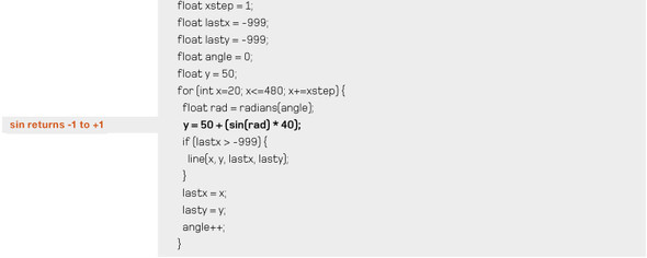
This code produces the curve shown in figure 3.7.

Figure 3.7. A sine curve

If you replace sin with a cosine function (see figure 3.8), the result is similar. Sine and cosine are used to calculate the points around a circle (more of that in the next chapter), so it’s unsurprising that the values they return are a nice smooth variance.

Figure 3.8. A cosine curve. Not too dissimilar from a sine curve.

Having set out to experiment with chaos, this smooth predictability may seem useless. But that’s only because the calculation is too simple. It doesn’t take many degrees of abstraction before it starts looking like the unpredictability of a random or noise function.

How does it look if you cube sin (see figure 3.9)?

y = 50 + (pow(sin(rad), 3) * 30);

Figure 3.9. A line constructed from the return values of sin cubed

Or, how about if you add a bit of noise too (see figure 3.10)? Is that cheating?

y = 50 + (pow(sin(rad), 3) * noise(rad*2) * 30);

Figure 3.10. sin cubed, with a soupçon of noise

This is the basic principle: by mixing up a few mathematical transformations, you can start to get interesting and unique lines. Let’s put this principle into action.

3.3.3. A custom random function

The problem with random, as you’ve discovered, is that it’s just too damn random. Perhaps if you can transform the randomness into something a little more predictable, it may have more aesthetic value.

First, let’s create a custom function:

float customRandom() {
  float retValue = 1 - pow(random(1), 5);
  return retValue;
}

Then, use this function where you calculate the y position:

y = 20 + (customRandom() * 60);

What you’ve done with this function is raise the random number to the power of five (see figure 3.11). If you were to square the random number, you’d get a returned value that tended more toward 0. If you were to raise it to the power of a half, the number would tend toward 1. Taking it further, raising it to the power of 5 (or, in the other direction, 0.1 as another example), you get a range of random results that are, well, less random.

Figure 3.11. The customRandom function in action. It isn’t quite as random as random.

You can experiment further with other transformations within this function. You can even rewrite it so it doesn’t use the random function at all—instead, come up with a calculation so convoluted that it appears random, the same way other pseudo-random functions work.

3.4. Summary

All we’ve done in this chapter is look at various different ways of drawing a single line: leaving behind the convenience of Processing’s built-in line function, and discovering more interesting possibilities by iterating through the line a pixel at a time. Through this mechanism, you can add some attractive flavors of variance, freeing your line from its mechanical perfection.

In the next chapter, having mastered the art of messing up a simple job like drawing a straight line, you’ll apply this technique to something a little more substantial. Prepare yourself to rediscover the joys of trigonometry, as we look at that simplest of shapes, the circle.