Chapter 2. Processing: A Programming Language for Artists

In this chapter you’re going to become a programmer. Although you don’t necessarily need to know a programming language to experiment with generative art, you’ll find it makes things a hell of a lot easier.

Obviously, one chapter probably can’t cover everything there is to know about any one language, but I’m confident that in around 30 pages, I can introduce all you need to start getting creative with code: from Hello World, through basic syntax and functions, to publishing your work for print, video, or mobile phones.

But first, if you plan to invest a significant amount of time in learning a tool, I feel I must justify the choice of programming language I’ve made for this book. Even constrained as you are to the toolset of the early twenty-first century, you have an abundance of software choices for experimentation with generative visuals. The options range from expensive professional tools (such as Flash and 3ds Max) to free online resources (like HasCanvas and Scratch). But your time is precious, and you could never hope to master them all. For your purposes, you need just one. The best one.

To narrow it down, I came up with a few criteria. The language has to be easy, powerful, extensible, and well supported. I also wanted it to be equally adept at producing generative visuals for print and video, not just the computer screen. Most important, though, I don’t want you to have to pay for it. Even with these demands, we’re still spoiled for choice. This book could just have easily been focused on openFrameworks (www.openframeworks.cc/), Context Free (www.contextfreeart.org/), Structure Synth (http://structuresynth.sourceforge.net/), NodeBox (http://nodebox.net/) or vvvv (http://vvvv.org/). And if you ever find yourself looking for a new toy to play with, you’ll have fun exploring any of these. But I’m assuming that, for now, you’re new to the world of programming, so you want something that suits an initial gentle learning curve while retaining the scope for advanced techniques and professional results. With this in mind, I propose that there is only one obvious choice: Processing.

The main reason I favor Processing, though, and the reason it warrants a book like this one at this point in its life cycle, is that I believe this one tool marks a significant advance in the democratization of programmatic art. To date, generative art has struggled to catch on outside of the realms of mathematics and computer science—fields that have never traditionally attracted those with more adventurous aesthetic obsessions. Processing is perhaps the first language to enable the creation of professional generative art by a general audience, not just computer scientists.

2.1. What is Processing?

Processing was conceived as a language for artists. It was developed as an open source project (initiated by Casey Reas and Benjamin Fry while at MIT) specifically intended to teach programming skills via the instant feedback of visuals. It’s built on a much more complex and powerful language, Java, but greatly simplified and applied. As it has grown in popularity, the simplicity of the core language has been enhanced with third-party libraries, enabling it to also be put to other more sophisticated uses: drawing in 3D, reading XML, talking to MIDI or Arduino, or interfacing with other APIs (Flickr, Twitter, and so on).

Mozilla, the organization behind the open source Firefox web browser, has announced Processing for the Web, a project proposal for porting the Processing language and environment to the open web, so it can integrate with standard technologies like JavaScript and HTML5’s Canvas tag. This would mean Processing could be run directly in the web browser, without a plug-in. Already, strides have been made in this direction with John Resig’s Processing.js project, which implements Processing in JavaScript. There are also implementations of Processing in Ruby (http://wiki.github.com/jashkenas/ruby-processing/), Clojure (http://github.com/rosado/clj-processing), and Scala (http://technically.us/spde/), all of which have emerged as grassroots projects, typically through the work of a single coder, in the last two years. They’re clear symptoms of the growing popularity of Processing and its potential for the future. The barriers for entry are dropping as the potential distribution opportunities are expanding.

Mastery of a programming language is perhaps the single significant barrier of entry to generative art. Although it may not be possible to pick up Processing instantly, the learning curve required to get started with Processing makes it accessible to a much wider range of technical abilities than other languages, while it still retains the power to be more than just a toy or learning aid. All tools, even the most basic, come with a learning curve. Your first efforts with a pencil will unlikely be great works of art; and although most of us are first introduced to handheld drawing implements as children, when our brains are most malleable, it may take years to master even this simplest of tools.

The programming language is at the other end of the complexity spectrum: it can’t be encapsulated into a neatly tangible physical object, it requires a highly sophisticated chunk of hardware to run it (and is useless without it), and it’s abstracted in a way that makes input and response not immediately apparent. Rather than the immediate feedback of sweeping a pencil against paper and seeing the line created, the process of write—run—amend (or write—run—debug) puts a gap between the artist and their work.

But, as previously mentioned, the Processing language, once tamed, can assist you in your art, and become your collaborator as well as your instrument. The programming language, with mathematical and logical aptitudes far beyond your own, can do all the heavy lifting and leave you to concentrate on the finesse.

New programmers will find that there is a logic to coding that becomes familiar with time, appealing to the ordering, categorical instincts of the left brain. I hope, for the non-programmers who have picked up this book, that by the time you’re finished with it, the idea of programming will hold no trepidation. After you’ve made friends with your tool and established a confident working relationship, you can get on to having some fun with your new collaborator.

2.1.1. Bold strides and baby steps

The starting point for these explorations, as well as the Processing download, is the Processing website (see figure 2.1). You can find the latest version at www.processing.org/download/. It’s currently supported for Mac OS X, Windows, and Linux. The screenshots used throughout these pages are taken from the Mac version, but the interface is nearly identical for all the supported platforms.

Figure 2.1. Processing.org: an invaluable resource for tutorials, reference, and discourse. It’s also the place to download the latest version of Processing.

Note that it’s worth checking back to the Processing download page occasionally, because revisions to the language are frequent. The application went through 161 versions prior to its 1.0 release in November 2008, and it continues to be updated and improved. There are also many other resources to be explored at www.processing.org, including some great getting-started tutorials by Dan Shiffman and Ira Greenberg in the Learning area, lots of code examples demonstrating various features of the language (again in the Learning area), and an active forum in the Discourse area. And while you’re bookmarking things, you might also like to add both my site (www.zenbullets.com) and the Abandoned Art site (www.abandonedart.org) to your list; where you’ll find the downloads for this book as well as many other generative artworks and the source code behind them.

The following section will introduce you to the technology, show you around the Processing Development Environment (PDE), and point out where to write your first line of code. If you’ve coded before, you may not need much more than this to get you started. But if you do, the rest of the chapter is a whistle-stop tour of the language essentials, written specifically with the beginner in mind. It will take you through the key concepts of Processing and programming languages in general, and arm you with everything you need to start experimenting. If you’re a beginner, this section is essential.

If you have programming experience but haven’t tried Processing before, you may skim these pages a little faster than the rank amateur. But every programming language has its idiosyncrasies, so it will be useful for you to learn how Processing uses concepts such as the frame loop, for example. If you’ve programmed Java or any ECMA-based language (ActionScript, JavaScript), Processing should come naturally to you.

One of the joys of open community projects such as Processing is that there is no shortage of free resources on the web in support of the product. If you find that the tutorials in this chapter don’t suit your pace, plenty of free options are available to help you. Again, I refer you to www.processing.org as a starting point.

Okay, you’ve said hello to Processing; next, let’s see if you can get Processing to say it back.

2.1.2. Hello World

After you’ve downloaded Processing, installed it, and run it for the first time, you’ll see something similar to figure 2.2.

Figure 2.2. (Left) The empty PDE window: the first thing you’ll see when you download and run Processing

This window is called the Processing Development Environment (PDE). Quickly, before blankpage paralysis sets in, let’s type something. Key the following in the main window:

ellipse(25, 25, 50, 50);

Then, click the Run button: What do you see? The output window should pop up (see figure 2.3). In it is a 100 x 100 pixel canvas within which has been drawn an ellipse, center point at coordinates 25, 25 (measured from upper-left), width and height 50 pixels. This is the visual programming equivalent of Hello World.

Figure 2.3. (Right) Hello World. The output window shows the result of your commands.

The single line ellipse(25, 25, 50, 50) drew a circle 50 pixels in diameter with its center at point 25, 25.

If you’re new to coding, in only one line you’ve already mastered two programming concepts. You’ve called a function (ellipse) and passed it a number of parameters (x, y, width, and height). You can think of a function as a service you use to perform a certain task. Sometimes you feed it parameters; sometimes it only needs to be called. It may give you a value back, or it may just perform the task it’s designed for—such as drawing to the screen. Later in this chapter, you’ll write your own functions; but before you get there, you’ll test a number of the core functions built into Processing, of which ellipse is but one. If you click the Help menu and select Reference, you’ll see a full list of the others. The reference is also online at http://processing.org/reference/.

 

 

2.2. Programmatic drawing

Everything you need to know to start programming in the Processing language is contained in this and sections 2.3 and 2.4 to follow. After reading all three, you’ll have the basics not just of Processing but also of programming in general. At their core, all programming languages boil down to the same types of structures: variables, loops, and functions. When you’ve got a grip on these concepts in Processing, you’ll find you have half an understanding of many other languages and will be the toast of your local chess club.

I appreciate that some of this may be a little unintuitive at first. If you feel you’re in unfamiliar territory as you wander through, I’d suggest you take this chapter very slowly. Code along as we go, and take the time to play around with trying every code chunk until you feel in control; only move on when you’re happy. There is no time limit, and your patience will be rewarded. Experienced coders are probably already speed-reading chapter 3 at this stage, so I’ll assume I’m not catering to them from here on.

From chapter 3 onward, there’s a lot of fun to be had with graphical programming, getting messy and breaking rules. But before you can break any rules, you have to learn a few of the rules you’ll be breaking. It’s tedious, I know; but remember that if you want to effectively insult a Frenchman, you’ll be a lot more effective at it if you’ve learned French first.

You’ll start with drawing a few simple shapes.

2.2.1. Functions, parameters, and color values

In the previous section, you downloaded Processing, typed your first one-line script, and published it to the output window. You’d called your first function (ellipse) and passed it a number of parameters (x, y, width, and height). Now, let’s try a few more.

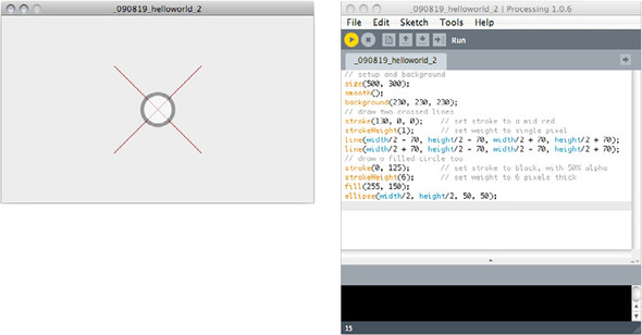
Open a new window, and type the following into the PDE window (see figure 2.4). Note that the lines beginning with // are comments, a place where you can put human-readable text. The // indicates that Processing shouldn’t try to run that line. You can also use the notation /* ... */ to spread comments across more than one line:

// setup and background
size(500, 300);
smooth();
background(230, 230, 230);
// draw two crossed lines
stroke(130, 0, 0);
strokeWeight(4);
line(width/2 - 70, height/2 - 70, width/2 + 70, height/2 + 70);
line(width/2 + 70, height/2 - 70, width/2 - 70, height/2 + 70);
// draw a filled circle too
fill(255, 150);
ellipse(width/2, height/2, 50, 50);

Figure 2.4. The PDE with your new script

Click Run, and you should see something like figure 2.5. What you’ve written in the PDE is a list of functions. I’ll walk you through them and explain what each one does.

Figure 2.5. The output window showing the result of the commands you’ve just written

First, set the size of the canvas to 500 pixels by 300 pixels:

size(500, 300);

Turn on smoothing, which anti-aliases the lines you draw so they don’t look jaggy:

smooth();

And set a grey background color:

background(230, 230, 230);

The three parameters to the background function are RGB values—Red, Green, Blue. Each value is a number from 0 to 255 defining how much of that color goes into the mix. Together, these three numbers give you 1.6 million combinations of colors you can use. In this case, because all three RGB values are the same, the result will be a grey color (any even mix yields a shade of grey). You can use a shorter version of the function for grayscale, with just one parameter: background(230);. This produces the same result as the three-parameter version.

Many other graphical applications use this RGB notation. If you’re unfamiliar with it, try a few different values from 0–255 in each of the background parameters to get used to this way of color mixing. You may also have seen hex values used to denote color values (as in HTML or Photoshop), such as #FF0000, which denotes red. This notation is similar; the three RGB values are expressed as hexadecimal (base 16) character pairs. Each two characters represent a color value: in the example, Red: 255 (ff), Green: 00, Blue: 00.^[1]

¹ For more information about hex notation, see www.web-colors-explained.com/hex.php.

You can use hex values in Processing if you prefer. background(#E6E6E6); produces the same result as background(230, 230, 230); (E6 hexadecimal = 230 decimal).

Next, let’s look at the stroke.

2.2.2. Strokes, styles, and coordinates

Returning to the code walkthrough, these are the next two lines:

stroke(130, 0, 0);
strokeWeight(4);

They tell Processing to set the color of your stroke (imagine this as your virtual pen) to a medium red (using RGB values again), and set the pixel thickness to 4.

After this, you draw a line in the stroke style you’ve just set:

line(width/2 - 70, height/2 - 70, width/2 + 70, height/2 + 70);

For this function, the parameters are (startx, starty, endx, endy); but in this case, you haven’t simply passed static values. In the slot for each of the four parameters is a simple sum. The result of each sum is passed as the parameter. Remembering that you previously defined a width and height of 500 x 300 pixels, you can calculate that the resulting drawn line will be from point (180, 90) to point (320, 220). (Coordinate values are always measured from upper-left.)

At this point, you may question why the function isn’t just written line(180, 80, 320, 220), because this would perform exactly the same action. The reason is that you’re trying to draw a cross relative to the center of the canvas. Yes, you know that your canvas is 500 x 300, because you set these values yourself only a few lines back; but if you use Processing’s knowledge of the canvas width and height, instead of relying on your human faculties, then if you go back and change the size function at any point—say, to size(600,150) (go on, try it)—the crossed lines will still meet at the center point.

An absolute coordinate (250, 150) never moves. But a relative coordinate (width/2, height/2) dynamically repositions itself relative to the size of the canvas.

The next line of code does the same, drawing a second line relative to the center point to complete the cross:

line(width/2 + 70, height/2 - 70, width/2 - 70, height/2 + 70);

This is a good point to introduce another programming concept: the variable.

2.2.3. Variables

You can see that you’re performing the same calculation (width/2 and height/2) multiple times. Wouldn’t it be neater if you did it only once? Your code will be easier to read, and it will execute faster if the processor has to do fewer calculations.

When you get into more complex coding, you’ll see that one of the biggest limitations is speed. The CPU in any machine can perform only so many calculations per second. It may not matter at this point when you’re managing just a handful of instructions; but it won’t be long until you’re performing many thousand calculations per second, so it’s worth developing a consideration of efficiency. If there is ever a way to easily reduce the number of calculations you’re performing, you should take it.

Try changing the two cross-drawing lines to the following:

float centX = width/2;
float centY = height/2;
line(centX - 70, centY - 70, centX + 70, centY + 70);
line(centX + 70, centY - 70, centX - 70, centY + 70);

Here you declare two variables to hold the result of a calculation. Think of a variable as a box in which you can put only one thing of a certain type; but the thing you put in may, um, vary (hence variable). You have to declare your box before you can use it, and give it a name (which can be anything you want), although you don’t necessarily have to put anything in it at first. The following is a valid way of declaring and filling a variable:

float centX;
centX = width/2;

You declare a variable by defining the type of data you’ll be putting in it, in this case a float. A float? “What’s a float?” I hear you cry. Table 2.1 lists all the built-in variable data types you have to choose from.

Table 2.1. The most common Processing data types

DATA TYPE	EXAMPLE OF USAGE	DESCRIPTION
char	char varName =’a’;	A letter or Unicode symbol, such as a or #. Note the single quotation marks used around the symbol.
int	int varName = 12;	An integer (a whole number). Can be positive or negative.
float	float varName = 1.2345;	A floating-point number. A number that may have a decimal point.
boolean	boolean varName = true;	A true or false value. Used for logical operations because it can only ever be one of two states. (It can also be undefined, but this would resolve as false.)
byte	byte varName = -127;	A less commonly used data type, which can only store a numerical value between -127 and 128. It’s most useful when you need to communicate with the serial port, which you won’t do in this book.
String	String varName = "hello";	A list of chars, such as a sentence. Note the capital S on String, signifying that this is a composite type (a collection of chars).

Next, let’s look at fill colors and alpha values.

2.2.4. Fills, alpha values, and drawing order

Okay, we’ve thoroughly deconstructed the drawing of two crossed lines. The final two lines of the script draw the circle:

fill(255, 150);
ellipse(width/2, height/2, 50, 50);

What you’re doing here, before you draw the circle, is setting a fill color. The fill is the area within the lines of a shape. Using this fill value and the stroke you previously set for the crossed lines, the final command draws a circle (an ellipse with equal width and height). You set the fill color using the single color value 255 (the grayscale notation), which is white. But you also have a second parameter that sets the alpha value—the transparency of the color—again, a number 0–255.

An alpha value of 0 is fully transparent, whereas 255 is fully opaque. Any time you define a color, you also have the option of giving it an alpha value. If you like, go back and try adding an alpha parameter to your stroke color too. With the three-parameter RGB syntax, the alpha value is the fourth parameter:

stroke(130, 0, 0, 50);

The order in which you’ve written the functions means that you first draw two solid lines and then place a semitransparent circle on top of them. The list of functions that make up the program are executed in the order they’re given. If you change the order so that the ellipse is drawn before the crossed lines, the point where they cross will be above the semitransparent white circle, so the lines will appear solid. Try the following code if you don’t believe me:

size(500, 300);
smooth();
background(230, 230, 230);

float centX = width/2;
float centY = height/2;
stroke(130, 0, 0);
strokeWeight(1);
fill(0, 40, 0);

ellipse(centX, centY, 30, 30);
line(centX - 70, centY - 70, centX + 70, centY + 70);
line(centX + 70, centY - 70, centX - 70, centY + 70);

The first section of the code sets up the drawing and creates the background. Next, you set the stroke and fill. Finally, you draw the circle followed by two lines.

The order of execution is relevant not only to the layering of your drawing but also to the styles you set. Processing is state-based, which means that when you set a style (such as the color or weight of the stroke), that state will be maintained until you set it to something else. In the example, you call stroke and strokeWeight before drawing anything, so all the lines drawn are of the same style. But you can change these settings as often as you please; whenever a line is drawn, it uses whatever setting was received last. Here’s an example that changes the stroke styles between shapes:

size(500, 300);
smooth();
background(230, 230, 230);

stroke(130, 0, 0);
strokeWeight(1);
line(width/2 - 70, height/2 - 70, width/2 + 70, height/2 + 70);
line(width/2 + 70, height/2 - 70, width/2 - 70, height/2 + 70);

stroke(0, 125);
strokeWeight(6);
fill(255, 150);
ellipse(width/2, height/2, 50, 50);

The result is shown in figure 2.6.

Figure 2.6. Commands such as stroke, fill and strokeWeight set the drawing style before a shape is drawn.

If you don’t want your ellipse (or any other shape) filled, you can use the function noFill (a function with no parameters) to remove the fill entirely. Similarly, if you want to turn off the stroke, call noStroke.

This covers the basics of drawing in Processing. Feel free to take a little time to try a few commands to get used to the coordinate system; or perhaps pick a few other shapes from the Processing reference, such as rect to draw a rectangle or quad for a non-right-angled quadrilateral. I’m not going to give you any clues as to what the triangle function might create.

Once you’re happy with your drawing skills, next you’ll learn a little more about how to organize code and control decisions, as we introduce animation.

2.3. Structure, logic, and animation

So far your scripts have been nothing more than a short list of instructions to perform, after which they stop. But with anything above the most basic level of simplicity, you need to go a little further: you need ways to group instructions and make decisions. It’s time to step it up a notch.

2.3.1. The frame loop

This section introduces a concept that is Processing specific (although it exists in many other tools too): frames. The word frame can mean a variety of things within the computer sciences, but our meaning is the movie industry sense—a single still image which, if we flash enough of them faster than the eye can see, gives the illusion of animation.

With Processing, a frame loop redraws the screen continuously. If you instruct Processing to do so, you can use this feature to add the dimension of time to your two-dimensional visuals and can create works that grow and move.

To enable this way of drawing to the screen, you need to begin putting your code in function blocks. A function block is a way of chunking a group of commands together. Processing sets aside two special blocks for frame-based scripting: setup() and draw(). The code inside the setup() function block is called once when the program launches, so it should contain all your initialization code—setting the canvas size, setting the background color, initializing variables, and so on. The code you write inside draw() is then called repeatedly, triggered on every frame. You can set the speed with which draw() is called by using the frameRate function. If you give it a number (12, 24, 25, and 30 are typical), it will attempt to maintain that rate, calling draw() regularly. Otherwise, it will perform the frame loop as quickly as the machine can handle.

Note that if you’re performing many complex instructions with every frame, your machine may not be able to process the code as fast as the frame rate you’ve specified. It will loop as fast at it can, which may result in not just a lower frame rate, but potentially an irregular one as well.

Let’s look at an example. Open a new script, and enter the code in the following listing. Don’t worry if you don’t understand all the instructions in the function blocks—a few more new concepts are being introduced here that you’ll step through in the next few pages.

Listing 2.1. Organizing code into setup() and draw() function blocks

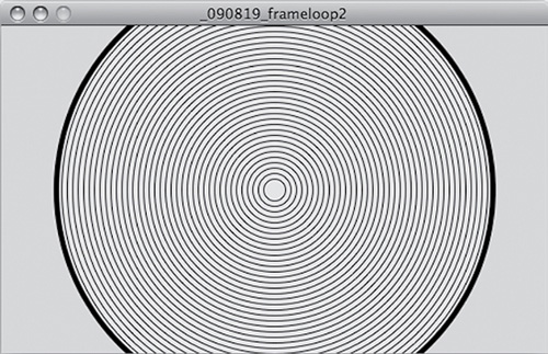
When you run this you’ll see a circle grow toward you in the output window, stopping when the diameter reaches 400 pixels (see figure 2.7). The diameter and the center points are kept in variables, with the center points calculated in setup(). The frame loop then checks that the diameter is smaller than 400, redraws the background, draws the circle, and increases the diameter by 10 for the next time it goes around the loop. The effect is that it draws a circle of diameter 10, 20, 30, and so on until the diam variable gets to 400. Note that the frame loop continues to be called over and over after the circle has reached its full size, but the draw() script is no longer drawing anything.

Figure 2.7. A circle drawn using a frame loop. When you run the script, the circle grows from a diameter of 10 to 400.

As soon as you start using function blocks, you lose the convenience of being able to write commands outside of function blocks, which is what you’ve been doing so far. But don’t look back—that capability was just a feature to improve the learning curve (thanks, Processing). You’re welcome to continue programming long lists of sequential commands if you choose, seeing how you’re so good at it now, but you can only go so far with that formatting.

Notice that you still declare your variables outside of the function blocks. This is fine syntactically: declaring variables outside of the function blocks means the contents of those variables are available to any and all function blocks in the script. If you define a variable within a function block, rather than outside it, that variable is only available within that block. It’s good practice to do this if a variable is only needed within a single function (then the processor doesn’t have to remember that value and can free up its memory for some other use).

This is called variable scope. Variables inside functions are called local: they only exist in that locality. Variables outside of functions are called global: they’re everywhere. A variable with an unintended scope is a common programming bug for amateurs and experts alike, so it’s one of the first things to check if your code is behaving unexpectedly. Many programmers use an underline (_) symbol to preface the names of global variables, so they don’t get confused. For example:

int _num = 20;
void draw() {
  int inc = 10;
  _num = _num + inc;
}

Here, the first line declares a global variable (_num), whereas the inc variable in the function block is local.

The chunk of script in listing 2.1 contains a number of other new concepts for the nonprogrammer. Before you continue playing with the frame loop, let’s look at those in more detail.

2.3.2. Writing your own functions

First there is the function block itself. The syntax of a function block is

returnType funcName([parameters]) {
  // code in here
 }

The return type of the setup() and draw() functions is void, which is Processing’s way of declaring that the function doesn’t return anything at all. There are no required parameters to these functions either. The other valid return types for functions are the same as the data types for variables: String, char, int, float, and so on.

The idea of a function returning something will make more sense when you start creating functions of your own. Open a new script, and try this:

void setup() {
 int x = AddNumbers(1,2);
 println(x);
}

int AddNumbers(int a, int b) {
  int returnValue = a + b;
  return returnValue;
}

The first function setup() is automatically called by Processing when the script is launched. But the second function AddNumbers is one of your own and won’t do anything until you call it. You do this within the setup() function: define an integer variable x, and set its contents to the return value of the custom function AddNumbers(1,2);. You define the return value of your custom function as an int also; otherwise, you’d get an error. You also define the data type of the two parameters the function requires, so it knows what to expect.

The custom function adds together the two parameters it’s passed, puts the result in a variable, and returns that variable. If you give a function a return type, there must be the keyword return somewhere within the function; otherwise it throws an error. After the function has completed its job and the returned value has been put into variable x, Processing continues to execute the commands in the setup() function block. The line println(x) outputs the value of this variable to the console window (the black window below the text editor in the PDE). This script has no visual output, so the output window is an empty canvas.

2.3.3. Operators

Within your custom function is another new programming concept: an operator, returnValue = a + b. Nothing to worry about here—it’s just math. The full list of operators is in table 2.2.

Table 2.2. Operators used in Processing

OPERATOR	NAME	EXAMPLE	EXPECTED RESULT
+	Addition	num = 45 + 5;	num becomes equal to 50.
-	Subtraction	num = 45 − 5;	num becomes equal to 40.
*	Multiplication	num = 45 * 5;	num becomes equal to 255.
%	Modulo	num = 45 % 5;	num becomes equal to the remainder of 45 / 5 (0).
/	Division	num = 45 / 5;	num becomes equal to 9.
++	Increment	num++;	The value of num increases by 1.
--	Decrement	num--;	The value of num decreases by 1.
+=	Add assign	num += 4;	Adds 4 to the value of num, and puts the result back in num.
-=	Subtract assign	num -= 4;	Subtracts 4 from the value of num, and puts the result back in num.
*=	Multiply assign	num *= 4;	Multiplies the value of num by 4, and puts the result back in num.
/=	Divide assign	num /= 4;	Divides the value of num by 4, and puts the result back in num.
-	Negation	minusnum = -num;	Multiplies the value of num by -1.

You can group your operators and define the order they’re dealt with by using brackets, just as you do in conventional mathematical notation:

float a = 45;
float b = 5;
float c = 4;
float sum1 = (a + b) * (b * c);
float sum2 = a / (b + c);

In this example, sum1 will contain 1000 (50 * 20), and sum2 will contain 5 (45 / 9).

Note that we use floats where the result of a sum may not necessarily be a whole number. There are also a few mathematical functions you’ll find useful:

• ceil()—Rounds up to the nearest whole number
• floor()—Rounds down to the nearest whole number
• round()—Rounds up or down to the nearest whole number
• min()—Returns the smallest of the list of numbers passed
• max()—Returns the largest of the list of numbers passed

The three rounding functions are most useful when you’re converting from floating-point numbers to integer values:

int centX = floor(width/2);

Without the floor() function, it would throw an error because if the width is an odd number of pixels, the result is floating-point number. The floor function prevents the error and ensures that you’re always dealing in nice whole numbers (and you’re not going to be able to see the difference if your center point is half a pixel off anyway).

The Processing language includes a lot more sophisticated math functions, some of which you’ll use later in this book’s experiments. If you want to leap ahead and try some of your own code-based fun, look at the available functions in the Processing reference and play around.

2.3.4. Conditionals

The final new element in the circle-drawing script is the conditional:

if (diam <= 400) { ... }

A conditional checks that a condition has been met before executing the code inside the block marked by the braces that follow it. In this case, the conditional asks whether the value of diam is less than or equal to 400. If it is, the code in the block executes. If not, the code in the block is skipped:

// check a condition
if (diam <= 400) {
   // execute code between the braces
   // if condition is met
}

You can also use an else clause to provide a block of code to be executed if the condition isn’t met:

if (diam <= 400) {
  // execute this code if diam <= 400
} else {
  // execute this code if diam > 400
}

If you imagine the flow of execution as a trickle of water running down the script, by setting a conditional you’re effectively creating different channels for the stream to follow. With an if ... else clause, the stream can go one of two ways. if on its own means the stream either goes through the block or goes around.

The comparison operators you can use are as follows:

• == equal to
• != not equal to
• > greater than
• < less than
• >= greater or equal to
• <= less than or equal to

You can also use logic operators to group conditions

• || logical OR
• && logical AND
• ! logical NOT

Here are a few examples:

String likeStr;
if ((likeStr == "pina colada") || (likeStr == "getting lost in the rain")) {
   println("come with me and escape");
}

Note also that conditions can be nested as deeply as you like. The following is valid code:

int man = 5;
int devil = 6;
int god = 7;
if (man == 5) {
   if (devil == 6) {
      if (god == 7) {
         goToHeaven("monkey");
      }
   }
}

But in this case, the same result can be achieved as follows:

if ((man == 5) && (devil == 6) && (god == 7)) {
   goToHeaven("monkey");
}

Now you’re starting to get the idea of programmatic flow and trusting the logic to make decisions for you. Next, in the final chunk of programming essentials, we’ll look at one of the few things our calculating machines can do better than us humans: repetition.

2.4. Looping

There is one last core programming concept you’ll need to in order to call yourself a coder: the loop. After that, we’re finished, I promise. The ability to take a single instruction or group of instructions and repeat it hundreds, thousands, or millions of times is a key advantage of programmatic drawing over any other comparable creative process. This is a very straightforward way to scale ideas.

You have already encountered one working loop in the previous examples: the frame loop. The chunk of code within the draw() function is called every time a new frame is entered, so the code is executed repeatedly for as long as the program is running. You can use this to perform repeating actions if you want, but this isn’t the only loop available to you. You can code your own loops, too.

Reload the circle drawing frame-loop script from a few pages back, and let’s try it.

2.4.1. While loops

A code loop looks something like this:

int bass = 99;
while (bass > 0) {
  println(bass);
  bass--;
}
println("how low can you go");

This outputs the value of bass to the console window 99 times. The while command checks a condition and, if the condition is met, executes the code inside the braces; it then loops back up to the top of the block. The execution continues to the final line only after the condition is no longer met (in this case, when bass is 0).

Note that if you don’t include the bass-- line inside the loop, which subtracts 1 from the number every time it loops, the condition will never be met and the loop will go on forever. This is one of those errors the compiler isn’t always clever enough to spot when you click Run. If your code includes an infinite loop, it can lock up your system, and you may have to force-quit Processing to escape it. So be careful out there, kids.

Let’s put this into action. Modify the circle script with the additions highlighted in the following listing, and then run it.

Listing 2.2. Drawing with a while loop

Here you have a loop within a loop. You copy the diam value into another variable; and then, every time you draw a circle of whatever diam you’re currently at, a second loop draws circles inward, decreasing the diameter back to 10 in 10-pixel jumps. You can see the effect in figure 2.8.

Figure 2.8. Circles within circles, a loop within a loop

Notice how you have to add extra lines to reset the stroke and fill; otherwise, the next time the frame loop was triggered, the previous settings would be applied.

2.4.2. Leaving traces

There is actually a much easier way of drawing concentric circles though. Try the following.

Listing 2.3. Concentric circles drawn using traces

int diam = 10;
float centX, centY;

void setup() {
  size(500, 300);
  frameRate(24);
  smooth();
  background(180);
  centX = width/2;
  centY = height/2;
  stroke(0);
  strokeWeight(1);
  noFill();
 }

void draw() {
  if (diam <= 400) {
 // background(180);  comment out this line
  ellipse(centX, centY, diam, diam);
  diam += 10;
  }
}

Again, you see the same concentric rings from figure 2.8, but with fewer lines of code. The crucial change is that you comment-out background(180);, the command that clears the image every frame (and forces you to redraw everything every time). If you don’t clear the image, you draw over the top of the previous frame. The animation of the growing circle is a series of frames of circles at growing diameters. If you don’t clear the frame, you can see the traces your movement leaves.

You can use this to great effect. Try changing the noFill(); line to fill(255, 25);, giving each circle a highly transparent white fill color (see figure 2.9).

Figure 2.9. By not clearing the frame every time you redraw, you can create subtle fades using alpha values.

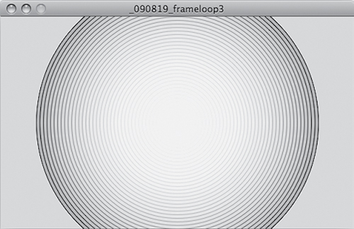
Even though the transparency is barely visible, the effect is accumulative. In the center, where more circles are layered atop each other, the white is deeper than on the edges where fewer circles are overlaid.

2.4.3. For loops

There is one final loop to show you before we can go boil the kettle. The for loop is used when you want to iterate through a set number of steps, rather than just wait for a condition to be satisfied. The syntax is as follows:

for ([initial state]; [end condition]; [step]) {
  code to be executed
}

An example is probably the best way to see how this works. Open a new script, and enter the following:

No frame loop this time, just a single block of code. The initial state of the for loop sets a variable h to 10. The code in the loop executes until h <= (height-15) (the end condition). Every time the loop is executed, the value of h increases by 10, according to the step you’ve defined (h += 10). This means the code inside the parentheses of the for loop will execute 28 times, with h set to 10, 20, 30 ... 270, 280.

Knowing that the h variable follows this pattern, you can use it in multiple ways. The lines you’re drawing are in 10-pixel steps down the canvas, because you use h for the y value. But the alpha transparency of the lines also varies as h varies: the black line gets lighter, and the white line gets darker (see figure 2.10).

Figure 2.10. Demonstrating the for loop in action

You can also terminate loops from within the code block using the break; keyword. For example, if you wish to stop your loop as soon as the black line is entirely invisible (and the white line is fully visible), place the following line inside the loop:

if (h > 255) { break; }

Okay new programmers, you now have a fistful of new concepts to get your heads around. There are a few more to come in later chapters, but these are the essential ones. Master these few, and you’ll have all the necessary skills to call yourself a coder and be able to hold your corner at a very boring dinner party.

Plenty more programming concepts may be new to you in the remaining chapters of this book, but we won’t dwell on them quite as long as we have here. If you’re still struggling to get your head around the logic of the procedural processing of instructions, I suggest that you take the time to experiment with the small set of concepts introduced in this section, and also make use of the many great free resources at Processing.org (in particular, the code examples in the Learning section).

Next, we’ll look at what you can do with your creations after you’ve finished coding them.

2.5. Saving, publishing, and distributing your work

The simplified syntax of Processing is perhaps its chief advantage, particularly for the amateur programmer; it greatly reduces the learning curve. But Processing also makes it significantly easier to publish your work and share it with the world.

Before you publish your work you should save it. Save, if you haven’t already worked it out, is the fifth button on the toolbar (see figure 2.11)—the down arrow. When you first save a script, a folder is created with the name you provide in the dialog box. Your script is saved as a text file in this folder, sharing the same name, with the extension .pde appended. The reason for the folder is to keep things neat when you begin importing and exporting.

Figure 2.11. The toolbar

You’ll notice that when loading and saving, Processing uses the term sketch to refer to the bundle of scripts and resources that go into a folder. I presume this is to increase the artist appeal, but I think the metaphor becomes rather limiting after a while. You’ll have to pardon me if I continue to refer to the text files as scripts and the bundle as the script folder. This way, you won’t end up sounding like an idiot if you ever find yourself having a conversation about similar concepts in some other programming language.

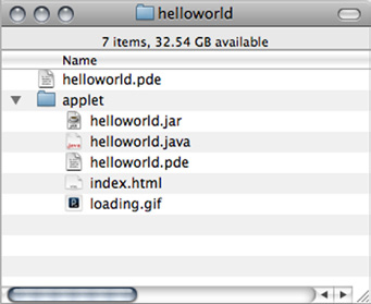
Once you have your script folder, you can free your pixels from the confines of the local output window in a number of ways. The first to try is clicking the Export button (the far-right arrow on the toolbar). Doing so creates a folder called applet within your script folder, containing everything needed to run the sketch in a web browser (see figure 2.12). If you launch the index. html file in a browser, there’s your creation, ready to be uploaded to the web (if that is what you want to do with it).

Figure 2.12. The script folder (sketch), containing the script (.pde) and an exported applet folder

 

 

To generate applications to run on the desktop, choose File > Export Application. This enables you to create standalone applications for OS X, Linux, and Windows, or all three at once. Again, the folder containing all you need for these installations is placed in your script folder.

2.5.1. Version control

Having shown you the handy Save button on the toolbar, I’m now going to advise you to stop using it immediately. A much more useful feature is available for organizing your work: Save As, which you can only access via the File menu (or using the keyboard shortcut Apple-Shift-S on the Mac). If you get into the habit of using Save As instead of just hitting Save, you’ll be prompted for a name every time you save. You can increment this name—HelloWorld_1, HelloWorld_2, and so on—leaving a version trail as you code.

This technique is called version control, and it’s useful to have in place to protect your work (it means you can always roll back to an earlier version). But it’s also useful for psychological reasons. If your work has a trail of iterations, it frees you to make more sweeping changes to your code, to take new directions, or to try stupid ideas, without worrying about doing anything catastrophic.

This will, imperceptibly, make your coding bolder and more confident, in the same way that when you drive a bumper car at an amusement park, you feel safe knowing that no one is really going to get hurt no matter how crazily you yank the wheel. You tend to drive more recklessly than you would the family sedan.

This practice also enables you to revisit interesting accidents or follow strange tangents. There is little overhead to saving multiple versions; the scripts are just text files (rarely more than a few KB), so they won’t fill up your disk.

This amazing feature may seem blindingly obvious to anyone new to coding, but you’d be surprised how this isn’t always easy to do in some other more sophisticated programming languages (usually because there are often many files with multiple dependencies upon each other). This is partly why different languages can have such different flavors. Some encourage a methodical, structured approach; while others, such as Processing (in its native PDE form, anyway), are more attuned to creative flurries.

2.5.2. Creating stills

The final destination of a generative art project isn’t always an application or animation, nor may it be intended for the computer screen—in which case you’ll be interested in other forms of output.

Capturing still images from an application is relatively straightforward. You can export screenshots of the output window in a variety of formats as the application runs. If you put the following function into your code, it captures a snap at that point and saves it in your script folder:

saveFrame("screen-####.jpg");

The #### is replaced with the current frame number when the file is saved, to ensure that Processing doesn’t replace the image every frame. If you want to save as .png, .tif, or .tga, these formats are supported; you just need to change the extension in the filename parameter. You can also add folder paths to the URL.

If you place a saveFrame function in the draw() frame loop and use the hash syntax for your filename, you’ll fill your script folder with a succession of sequentially named image files. If it’s just a single image you’re after, you’ll end up with a folder full of imagery that you’ll need to sort through at some stage; so you may want to consider writing a conditional (an if statement) to snap an image only if certain criteria are met. It will likely require some pretty complicated logic for the machine to determine a good shot from a bad one, so the best way to capture the perfect still is probably to rely on your own eye instead. Include this function within your code:

void keyPressed() {
  if (keyCode == ENTER) {
   saveFrame("screen-####.jpg");
 }
}

The keyPressed() function is a built-in event function, called whenever a key is pressed. The previous function checks whether the key pressed is Enter and, if so, takes a snapshot and saves it in the script folder.

2.5.3. Using a still as an alt image

If you’re creating work for the web, here is a useful tip. You may have noticed in figure 2.12 that when you export an applet, it includes a loading.gif image file, which the browser displays while the application is loading or if it fails to load. If a user’s Java is incompatible, the loading image may be all they see; so a nice touch when delivering your works to the web is to replace this loading image with a still of the work that is loading. You do this by modifying the generated index.html file. Look for this line:

<param name="image" value="loading.gif" />

If you replace loading.gif with a reference to your own image, it provides a failsafe for users whose browser isn’t capable of running the Java application. At least they’ll see a still of your work, even if they can’t see it in action.

Next up: the moving image as an output format.

2.5.4. Creating video

A saveFrame function within the draw() loop creates a folder full of screenshots of every frame in a running application. What’s more, the image files are numbered sequentially if you use the hash syntax for your filename. This is useful for software such as QuickTime Pro, which can open an image sequence (available from the File menu in QuickTime Pro) to create a movie file.

The joy of creating for video is that you no longer have to worry about processing power and maintaining a smooth frame rate in Processing. Even if you’ve specified a frame rate using the frameRate parameter, the sketch will only run as fast as your machine allows. If you’ve overloaded it with some processor-heavy fractal-generation algorithms (which you will in part 3 of this book, believe me), a running application can still crawl. But if you export each frame as an image, to use video as your final medium, you have to take frame rate into account only when you build the movie from the image sequence. The movie will run as fast as you tell it, even if the image sequence it was generated from took many hours to create.

It’s common, when creating work for video, to leave a dedicated machine rendering frames overnight, and only see the result when you import the generated frames into your movie maker the next day. Obviously, this removes the immediacy of feedback that you’ve become used to when working with software, and you can start to get an appreciation for the computer scientists of previous generations who coped with programming via punched cards and mainframe computers. For more complicated movies, you’ll probably find yourself developing a system of working with wireframes—simplified or abstracted versions of the finished piece—while you develop, and only upping values/reenabling textures/knitting together features when you run a render.

If you don’t have (the incredibly useful) QuickTime Pro or a similar application capable of sequencing images into a movie, Processing can create QuickTime movies from within your code using the Video library, which also enables the use of a webcam as an input device. We won’t be covering the huge range of available Processing libraries in these pages, as it’s a topic worthy of a book in itself, but they aren’t difficult to use. You can explore the functions provided by the Video library at www.processing.org/reference/libraries/video/.

2.5.5. Frame rates and screen sizes

Processing snaps frames at whatever size you’ve specified for the stage, so a movie can be any dimension. Similarly, the frame rate you specify when importing the sequence is usually arbitrary. But there exist various standards that are used for the web and broadcast media.

When it comes to frame rates, 25 fps (frames per second) is the most common for work intended to be viewed on computer monitors or TVs, although 24 fps and 30 fps are also used in the US (this is the main difference between the 24 fps NTSC format of video that is standard in the US, and 25 fps PAL/SECAM used elsewhere). HDTVs use higher frame rates of 50 or 60 fps because it’s been proposed that somewhere around the 50-60 fps mark is the limit of flicker-fusion—the point where the human eye can’t tell it’s watching frames. If you imagine a movie as being alternating black and white frames, at frame rates below 50-60 fps, a person would see it as a flicker; above this limit, it would be seen as grey. This said, a certain amount of lo-fi flicker isn’t prohibitively uneasy on the eyes, and an animation can still look smooth at a frame rate of 12 or so.

With screen dimensions, a widescreen format is the most common, usually a 16:9 ratio (such as 1024 x 768 or 1280 x 720). The best practice, though, is to consider where you may want to show your video, and aim for that. Projecting a work onto the wall of an art gallery will doubtless require a different screen ratio than a work designed for mobile phone.

If you’re creating video for the web, screen, or TV, the 16:9 standard is pretty ubiquitous. YouTube, for example, currently recommends 1920 x 1080 or 1280 x 720. If you don’t use the 16:9 ratio when you upload to YouTube, black borders are automatically added to your movie, padding it to fit. Vimeo isn’t too dissimilar, currently supporting 640 x 480 standard definition, 853 x 480 widescreen DV, and 1280 x 720 HD.

2.5.6. Mobile devices, iPhone/iPad, and Android

Processing, as you’ve discovered, is based on Java. Most modern mobile phones run Java. Does this mean you can create mobile-phone applications in Processing? The answer is yes. Kinda.

If you wish to develop for devices that use Google’s Android operating system, it couldn’t be simpler. Processing enables you to publish sketches to an Android emulator or an attached device as easily as you can export them to the desktop. The 1.5 release of the Processing IDE added a new button to the toolbar, which toggles the view between “Standard” and “Android”. If you select Android Mode, the run and export functionality will be overridden to target a device. You will need to have the Android SDK installed on your machine to use this though. Full instructions on how to set this up are at http://wiki.processing.org/w/Android. There are also two great tutorials on creativeapplications.net that talk through the creation of your first Android app^[2] and publishing it for the Android Market^[3], by Jer Thorp and Jerome Saint-Clair respectively.

²http://www.creativeapplications.net/android/mobile-app-development-processing-android-tutorial/.

³http://www.creativeapplications.net/android/from-processing-to-the-android-market-tutorial/

If you’re targeting a wider range of devices, including older mobile phones, Processing also has this capability, but it’s not as fully featured as the Android route. The Java that most current mobile phones run is special flavor called Java Micro Edition (Java ME), which means there is a special flavor of Processing too to go with it. Mobile Processing isn’t a library but an entirely separate application. It has a stripped-down subset of Processing’s functions but includes extra functions for dealing with touchscreen interaction, memory management, and other functionality that’s specifically relevant to mobiles. It has a similar IDE, but you also need to download a wireless toolkit (WTK)—basically, a phone emulator—to develop for these very particular mini platforms.

I won’t go into further details here but will only say that, yes, if mobile is a platform you want to target, the majority of the material in this book can be applied to Mobile Processing as easily as it can Processing. To get started, you can download the IDE and WTK from http://mobile.processing.org/download/. As with Processing, the project is well supported, and a number of tutorials and a reference are available on the site to get you started.

The iPhone and iPad though, are a different matter. When the iPhone was launched in the UK, the Advertising Standards Authority banned an Apple advertisement that claimed the iPhone gave you access to “all the internet,” on the basis that if a device doesn’t run Java or Flash, it can’t really claim to cover “all the internet.” At the time of writing, neither Java nor Flash runs on the iPhone, either natively or in the web browser. To develop for Apple platforms, you need to learn Objective-C and be prepared to pay to publish through Apple’s App Store.

This situation may, I hope, change over time. Small steps are already being made. But at the time of writing, the huge success of the iPhone, iPad, and the App Store doesn’t really put any pressure on Apple to encourage development using other technologies. Recent versions of Flash include a compiler to create iPhone apps, even though Apple’s Terms and Conditions prohibit its use. There is also a comparable, and promising, initiative for Processing, called iProcessing. But non-native conversions from one language to another will never compete with native Objective-C applications in terms of performance.

If you want a quick way to see your Processing sketches on your iPhone, there is one beautifully crazy solution. I’ve already mentioned Processing.js, the JavaScript port of Processing. It’s quite a little marvel. It uses HTML5’s Canvas element to draw shapes directly in the web browser. Like Mobile Processing, it supports only a subset of Processing functions, but it has the added power of being able to mix JavaScript and Processing code together (they’re similar in syntax).

You can find the download and introduction to Processing.js at www.processingjs.org/. It exists as a few hundred lines of JavaScript that you include in a webpage. You’ll need a little experience with using JavaScript within HTML to get it working in your own web pages; but if you aren’t blessed with such skills, you can get straight into Processing.js via HasCanvas, an online interface developed by Robert O’Rourke. It enables you to program direct to the HTML5 Canvas tag in real time. You can find it here: www.hascanvas.com/. Anything you create using Processing.js can be seen just about anywhere you can view the web, including your favorite irritatingly proprietary but highly fashionable devices.

2.6. Summary

This brings you to the end of your introduction to Processing. You now have a tool grasped firmly in your eager little fists and are ready for some creative coding. You have the basics of programmatic drawing and a variety of options for media in which to publish—web, print, video, or mobile device. You’ve also learned a set of programming principles that will serve you well with any programming languages, not just Processing.

Next, we’ll bring the focus back to how you create art in the generative style. In chapter 3, we’ll look at randomness, noise, and the ways you might go about shrugging off the precise computer way of doing things and allow the pen to slip from your fingers a little.