Chapter 5. Adding Dimensions

Imagine you’re a tiny creature clinging to the surface of a large ball.^[1] You walk the surface of that ball for a lifetime, until you feel you’ve covered every part of its surface and know it intimately. At this stage, it feels as though there is nowhere new for you to go, nothing new to see. That is, until you discover up, and suddenly you find a perspective from which everything looks very different.

¹ This shouldn’t be hard to imagine, given that you actually are.

Often, we meet barriers like this in our work, when it seems there is nowhere else to take an idea. This is the point at which you should consider adding extra dimensions. If you’ve been working in one dimension, try it with two. If you’re working in two dimensions, try three.

The computer monitor, printed page, or gallery wall has only two dimensions. Anything you create for these media will always be flattened for presentation. But that doesn’t mean your work is limited to those dimensions. You’ve already learned, in chapter 2, how to make your work animate, giving it an extra dimension: time. In this chapter, we’ll revisit that idea, as well as learning how Processing renders three-dimensional drawing.

We’ll keep Perlin noise as our focus while we examine these concepts, because there is still much more to explore in relation to that subject. So far, you’ve only used the noise function with a single parameter, creating one-dimensional noise. You’ll begin by adding an extra dimension to that.

5.1. Two-dimensional noise

Noise in two dimensions isn’t much more complicated than it is in one—it’s just a matter of shifting perspective, conceptually, from a line to a plane. One-dimensionally, a progression of noise values yields a wavering line, like a mountain range viewed on the horizon. Looking at it in two dimensions, you’re viewing the mountain range from above, as if you were flying over it in a helicopter; looking straight down, you see a plane of peaks and troughs.

5.1.1. Creating a noise grid

The best way to demonstrate is with an example. Open a new script, and tap in the contents of the following listing.

Listing 5.1. A two-dimensional noise grid

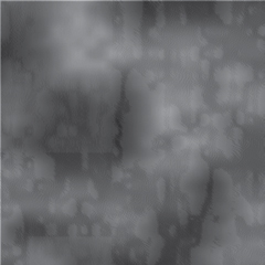
In this script, you create a grid of points (except I’ve used tiny lines instead of points, because in Processing lines are better at alpha values). You loop through the pixels of this 300 by 300 square, traversing column by column, row by row, one pixel at a time. Noise seeds in the x and y direction are incremented by 0.01 with every pixel, remembering to reset the x seed to its original position at the end of each row, like hitting the carriage return on an old typewriter. The return of the noise function for each x and y position is visualized as a variance in the alpha values on the tiny line you’re drawing at every position. The result is shown in figure 5.1.

Figure 5.1. Perlin noise in 2D, visualized as alpha values

The fun with two-dimensional noise is in dreaming up new ways to visualize it, which is what we’ll do next.

5.1.2. Noise visualizations

First, knowing that the two-loop traversal through the grid won’t change much, you can separate the visualization part into a function block. It will help if you also space the grid out a little, too, so you can see what’s going on.

Listing 5.2. The noise grid, rewritten into neat function blocks

The custom drawPoint() function takes three parameters: x and y to define where the point is, and the two-dimensional noiseFactor that has been calculated for that point. In this case, you draw a tiny square, using the noise factor to determine its size. Click run, and you’ll be looking at something like figure 5.2.

Figure 5.2. 2D Perlin noise visualized as squares of varying size

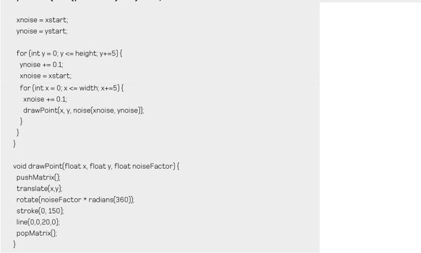
Now that you’ve defined the function, you can modify this part to experiment further. How about visualizing the noise as a rotation? Here’s a new version of the drawPoint function that draws a 20-pixel line rotated according to noiseFactor:

void drawPoint(float x, float y, float noiseFactor) {
  pushMatrix();
  translate(x,y);
  rotate(noiseFactor * radians(360));
  stroke(0, 150);
  line(0,0,20,0);
  popMatrix();
}

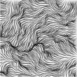
To perform the rotation, you used translate(x, y) to move the drawing position, and then you start the drawing from point 0,0 instead of point (x,y). You do this so the rotation is around the point you’re drawing at, not the upper-left 0,0 point. The functions pushMatrix and popMatrix are a way of storing the previous drawing position before you perform the translation and rotation, and then restoring it afterward. Figure 5.3 shows the result.

Figure 5.3. 2D Perlin noise visualized using rotation

Okay, one more. Change background(255) to background(0) in the setup function, and then rewrite drawPoint so it varies the rotation, size, color, and alpha, all using the same noise factor:

void drawPoint(float x, float y, float noiseFactor) {
  pushMatrix();
  translate(x,y);
  rotate(noiseFactor * radians(540));
  float edgeSize = noiseFactor * 35;
  float grey = 150 + (noiseFactor * 120);
  float alph = 150 + (noiseFactor * 120);
  noStroke();
  fill(grey, alph);
  ellipse(0,0, edgeSize, edgeSize/2);
  popMatrix();
}

The resulting grid now looks something like figure 5.4.

Figure 5.4. 2D Perlin noise as little fluffy clouds

 

 

You get the gist. I’d suggest that you try throwing a few of your own ideas at this function to see what emerges. Perhaps have a rifle through the Processing reference to come up with different ways of drawing that you haven’t tried before, and then see how they can be subverted by applying the noise factor.

Next, we’ll look at time as an extra dimension, and see how you can apply noise to that.

5.2. Noisy animation

The frame loop, Processing’s built-in draw function, enables you to create images that change over time. This, folks, is what we call animation: you may have heard of it. Refer back to section 2.3.1 if you need a refresher on how the frame loop works. The following listing uses the draw function to turn the two-dimensional noise grid into something that moves.

Listing 5.3. Noise grid again, now drawing on the frame loop

 

The drawPoint function is unchanged, as are the x within y loops to traverse the grid. What’s new is that with every frame, you increment the start point for both the x and y noise seeds. When you run this, you’ll see something very similar to figure 5.4; but now clouds are drifting diagonally across the screen, as if a steady wind were blowing from the southwest. There are no moving parts—the illusion is created by scrolling across the noise plane.

Obviously, it’s a little difficult for me to demonstrate this in print, so you’ll need to be coding along to appreciate the effect. This movement seems a little predictable for my liking, though. If only there were some way to produce a smooth, natural variance. Take a look at the next listing.

Listing 5.4. Noise grid with noise variance added to the movement

The extra code before the grid loop uses two (one-dimensional) noise sequences to give a drifting camera position, floating over the noise plane with the gentle irregularity of a leaf in an updraft. You’ll notice for this example I rolled back the drawPoint function to the rotating-lines version from the previous section. Adding time to this particular visualization produces a nice illusion of ruffling fur, or the wind blowing through grass. Run it to see it in action.

Note that there is no limit to the number of noise sequences you can have in a single script. Listing 5.4 has four: xnoise and ynoise, which are combined to get a two-dimensional value; and xstartNoise and ystartNoise, which each give one-dimensional directional movement.

Next, we’ll explore new depths, as you learn how Processing draws in 3D.

5.3. The third dimension

When you use the size function to specify the canvas area, there is a third, optional, parameter—MODE—that you haven’t needed to know about until now. This is how you tell Processing which rendering engine to use:

size(width, height, MODE);

Table 5.1. Processing’s choice of renderers

MODE VALUE	DESCRIPTION
JAVA2D The default.	The highest-quality 2D renderer.
P2D (Processing 2D)	A faster 2D renderer, optimized for pixel data, but not usually as accurate as JAVA2D.
P3D (Processing 3D)	A fast 3D renderer, intended for Java on the web. Prioritizes speed and file size over quality.
OPENGL	A better high-speed 3D renderer that utilizes OpenGL graphics hardware, if available. OPENGL smoothes all graphics, so smooth and noSmooth commands become redundant. You need to import the OpenGL library to use this renderer (see listing 5.5).
PDF	A renderer for writing directly to PDF files, rather than the screen. This is ideal for drawing high-resolution vector shapes, particularly when you’re creating prints bigger than the screen (when you’d need to save to a file to see the results anyway). Requires the PDF library. For more information, see http://processing.org/reference/libraries/pdf/.

The list of renderers is in table 5.1. The default is JAVA2D, which produces the best two-dimensional images; this is what you’ve used up until this point. To draw in 3D, you’ll need to change MODE to either P3D or OPENGL. OPENGL usually gives better-looking results, but only P3D produces an applet small enough to publish to the web. For the purposes of this chapter, it doesn’t matter much which you choose.

Now, if you’ve chosen a renderer, let’s try drawing something.

5.3.1. Drawing in 3D space

You’re by now quite familiar with two-dimensional Cartesian coordinates, which is how you measure x and y positions on the canvas. To draw in 3D, you need to add an extra position—a z value—to measure how far you are above or below the 2D plane.

As with 2D drawing, Processing has a number of built-in functions for common 3D structures. You can begin using these to get a sense of drawing in a three-dimensional space. For this first example, you’ll use sphere. You’ll do the drawing using translate to move to a 3D position and then drawing relative to that point. You’ll find this is the only sensible option when dealing with x, y, and z coordinates.

Open a fresh window, and type the following:

import processing.opengl.*;

size(500, 300, OPENGL);
sphereDetail(40);

translate(width/2, height/2, 0);
sphere(100);

The first statement imports the OpenGL library. This line is added automatically if you import the library via the Sketch menu (Sketch > Import Library). The size command then sets the canvas size and selects this renderer.

Next, the sphereDetail command tells the renderer how much detail to use when drawing a sphere. 3D renderers can’t draw smooth curves, so any shape will always be made up of a collection of flat planes. By giving this command a value of 40, you effectively tell the renderer to make a new edge every 9 (360/40) degrees.

The final two lines create the sphere by moving the drawing point to the middle of the canvas and drawing a sphere around that point with a radius of 100. Notice how you pass three variables to the translate command, but you aren’t using z yet. The output is shown in figure 5.5.

Figure 5.5. A sphere drawn using OpenGL

So far, barring the lines, this doesn’t look too different from a circle created using the 2D renderer. But if you start modifying the third parameter of translate, you’ll see the difference. Change that line to translate(250, 150, 50); the sphere now appears bigger. You’ve moved it 50 pixels closer to you (a value of -50 moves it further away). If you set the third parameter to 150 it will appear as if you’re actually inside the sphere.

Let’s now use this new perspective to look at the 2D noise plane from the last section from a fresh angle.

5.3.2. Three-dimensional noise

Begin by entering the code from the following listing into a new window.

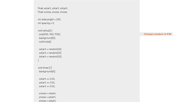
Listing 5.5. 2D noise from a 3D perspective

import processing.opengl.*;

float xstart, xnoise, ystart, ynoise;

void setup() {
  size(500, 300, OPENGL);
  background(0);
  sphereDetail(8);
  noStroke();

  xstart = random(10);
  ystart = random(10);
}

void draw () {
  background(0);

  xstart += 0.01;
  ystart += 0.01;

  xnoise = xstart;
  ynoise = ystart;

  for (int y = 0; y <= height; y+=5) {
   ynoise += 0.1;
  xnoise = xstart;
  for (int x = 0; x <= width; x+=5) {
   xnoise += 0.1;
   drawPoint(x, y, noise(xnoise, ynoise));
  }
 }
}

void drawPoint(float x, float y, float noiseFactor) {
 pushMatrix();
 translate(x, 250 - y, -y);
 float sphereSize = noiseFactor * 35;
 float grey = 150 + (noiseFactor * 120);
 float alph = 150 + (noiseFactor * 120);
 fill(grey, alph);
 sphere(sphereSize);
 popMatrix();
}

Aside from the change in renderer, this is similar to listing 5.4. The main difference is to the drawPoint function. Instead of translating to a 2D point, you translate to a 3D point. The code reuses the y value for the z depth as a shortcut; doing so creates a tiered square, sloping backward like theatre seating. At each 3D point, you create a sphere with a radius, fill color and alpha relative to the noise value. The result is another gently moving cloudscape, but with a better perspective (see figure 5.6).

Figure 5.6. Two-dimensional noise, three-dimensional perspective

The perspective is three-dimensional, while the plane you’re looking at, and the noise sequence that defines it, remain essentially two-dimensional. But the noise function can take up to three parameters, so you have the capability to generate noise in three dimensions. The visual metaphor for three-dimensional noise will no longer be a mountain range: now you need to imagine a cloud, or a smoke-filled room, and consider how you might use that type of variance to create visualization. You can begin by building a controlled block of this noise.

You’ll need to make a few changes to the loop. You’ll now be iterating through all the points in a cube rather than a plane, and so you’ll pass four parameters to the drawPoint function: x, y, z and the three-dimensional noise value for that point. The changes are made in the next listing.

Listing 5.6. Constructing a cube of three-dimensional noise

The cube you build is made up of almost-transparent boxes, the color of which varies by the three-dimensional noise factor. It’s still difficult to see, which is why you need the code to spin it around. You’ve essentially created a cloud in a box (see figures 5.7 and 5.8).

Figure 5.7. Three-dimensional noise: a cloud in a box

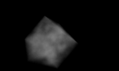
Figure 5.8. The source code for Haunted Fishtank (Abandoned Artwork #49), available at http://abandonedart.org/?p=449, is similar to the system you’ve developed in this section.

Calculating your way around three dimensions isn’t straightforward: the math of 3D space is considerably more complicated than traversing a 2D canvas. But it comes with practice. After you’ve played with it a while and got the hang of it, you may consider taking the “break it down, build it back up” approach of the previous two chapters and trying it with 3D shapes. By way of example, we’ll end this chapter with a quick look at the trigonometry of a sphere.

5.3.3. The wrong way to draw a sphere

Below are the not-so-magic formulae for plotting points on the outer edge of a sphere. They’re similar to the formulae for points on a circle (see chapter 4), but they require two angles (s and t) to determine a location relative to the center point:

x = centreX + (radius * cos(s) * sin(t));
y = centreY + (radius * sin(s) * sin(t));
z = centreZ + (radius * cos(t));

To construct a sphere without using Processing’s sphere function, you’ll take the same approach you did in section 4.1: iterate around rotations of these two angles. In doing so, you can project a line to every point on a sphere’s outer surface.

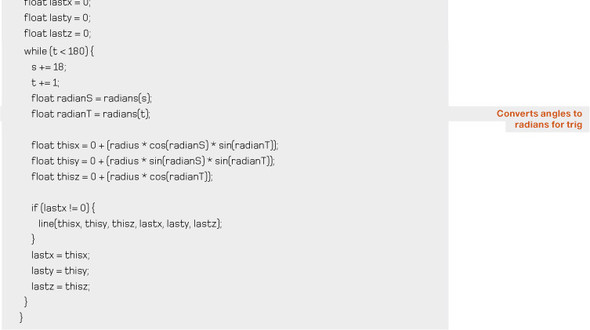
See the following listing for one application of this technique. The t angle circles around the central axis many times in 18-degree jumps, while the s angle does one slow 180-degree rotation turn.

Listing 5.7. Spiraling around a sphere

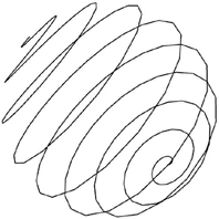
The result is a spiral drawn onto the surface of a virtual sphere, as shown in figure 5.9.

Figure 5.9. Spiraling around a sphere

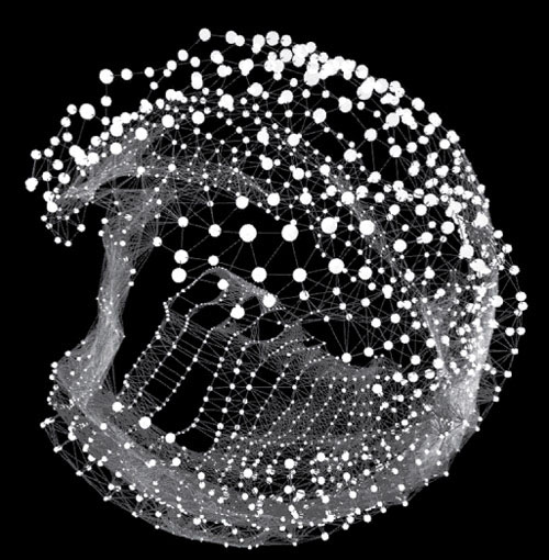
The three lines of trig at the beginning of this section have served me well in my own work. They’re the core math wizardry behind my video piece Frosti (2010), for example (see figure 5.10). I leave you with this magic to make your own, to take and pervert into your own creations.

Figure 5.10. Frosti (2010). A video work created by applying Perlin noise to a deconstructed sphere: http://vimeo.com/9712740

5.4. Summary

When an experiment feels like it has no further to go, you can always try adding an extra dimension. Be it a dimension in space or time. In this chapter, we’ve tried both. We’ve also introduced three-dimensional drawing in Processing, which can now be considered an extra string to your bow.

We have now, in this and previous chapters, pretty much exhausted Perlin Noise. Hopefully you now have a good appreciation of the range of effects you can produce with it. Anywhere we need a nice naturalistic variance it can be employed, which makes it such a useful convenience it is never going to fall too far down the toy box. I imagine it would be possible to spend a lifetime coming up with new ways to visualize this single algorithm, and when you tired of it you can change algorithm and waste a second lifetime.

As far as this book is concerned, we’re putting down the noise and random functions for a while so we can look at a more organic way of exploring unpredictability. In part 3, we’ll introduce an even cooler mathematical toy: emergence. We’ll look at the simulation of natural processes, and practical ways of evoking natural forms the way they’re constructed in the world outside of our laptops.