Chapter 8. Fractals
To my mind, there is something very “seventies” about fractal art. Even before James Gleick’s hugely popular book Chaos: Making a New Science (1987), which popularized the mathematics of chaos theory, fractal imagery, in particular the Mandelbrot set, was overly familiar from the kind of posters you might expect to see on the walls of hippie math grads.
We’ll never know why the renderers of early fractal art favored such lurid, psychedelic colors, but I assume it had a lot to do with the overconsumption of LSD. Anyway, I want this preconception of fractal art flushed from your mind as we explore self-similarity in this chapter. Fractal art can also be subtle and beautiful (see figures 8.1 and 8.2).
Figure 8.1. After experimenting with fractal structures, you’ll start to notice self-similar recursion everywhere. This illustration is from Ernst Haeckel’s 1904 book Kunstformen der Natur (Artforms of Nature)
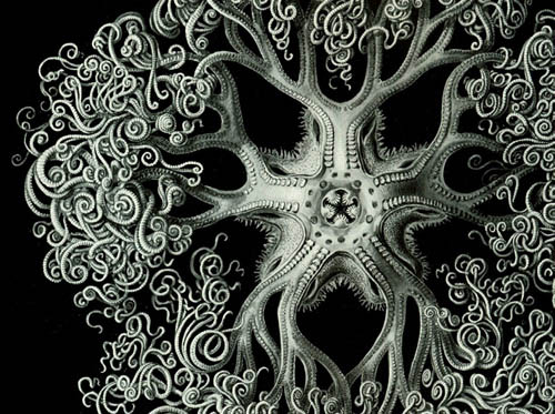
Figure 8.2. Mandelbulb by Tom Beddard (2009), www.subblue.com: a 3D version of the Mandelbrot fractal. See Beddard’s site or www.skytopia.com/project/fractal/mandelbulb.html for the math.

The code will be a little more involved in this, the book’s final chapter, pushing the object-oriented organization we introduced in chapter 6 as far as your processors will allow. But this is about as difficult as generative art ever needs to get. If you can wrap your head around a self-similar recursive fractal structure and re-create it in code (a feat you’ll be performing with great aplomb in a few pages’ time), you’ll find harnessing physics libraries, mechanical systems, fluid simulation, particles, AI, audio reactive art, or whatever explorations you want to pursue after you put this book down, won’t present any barriers to you.
Fractals, from the Latin fractus (meaning “broken”), are shapes or patterns that repeat at many levels. The patterns don’t necessarily need to be identical at the different scales; they just share certain types of self-similar structures. As with emergent patterns, fractal structures are everywhere in nature: in snowflakes, tree branches, rivers, coastlines, and blood vessels. The leaf of a fern is one particularly good example (see figure 8.3), where the fronds of each leaf mirror the shape of the leaf as a whole. Examine the frond in closer detail, and you’ll see that its subdivisions are the same shape again. This self-similarity repeats, continuing downward in scale, beyond the limits of the human eye.
Figure 8.3. Ghost Ferns (photographed by Flickr user L’eau Bleue:) fractal structures in nature

In this chapter, we’ll look at fractal iteration as a way of creating art. You’re already familiar with recursion: for loops, while loops, and draw loops. But this is a different breed of iteration, a reflexive iteration—a type that, unchecked, tends toward the infinite.
8.1. Infinite recursion
Imagine you’re standing before a mirror, with a second mirror behind you. You see a reflection of a reflection of a reflection of a reflection, onward toward the limit of perception. Strange things happen when you have an infinite recursion like this. Small changes, micro-movements, become massively amplified within this closed loop. Try holding a flame in such a mirror loop (go on, put the book down and try it—it’s really cool). The micro-randomness of the flame’s flicker creates bizarre abstracts as it’s repeated an infinite number of times. In the same way as the small interactions between many agents gave rise to an emergent complexity in the previous chapters, small changes in infinite, self-similar structures create a similar complexity, but on a more ineffable scale.
A computer can’t deal with the concept of infinity. You can’t ask a computer to loop an infinite number of times because, as a blind obeyer of instructions, it will never stop—the computer will loop for ever until you interrupt it or turn it off. This is Alan Turing’s halting problem: he proved that in addition to it being impossible for an infinite loop to ever return a result, it’s also impossible to determine in every case whether any given set of instructions will result in an infinite loop or reach a final state. This is one of the central concerns of the field of AI, that ultimate form of complexity we’re gingerly skirting around in these chapters. Telling whether a problem is finitely soluble or not is something a human can do instinctively, but this ability can’t be easily simulated by machines.
For example, you can tell at a glance that the following code will never reach a state where it stops:
int x = 1;
while (x>0) {
  x++;
}
This is an example of an infinite loop. It’s perfectly syntactically correct, but it will lock the processor into a never-ending cycle until something interrupts it. Infinite loops are easy to code but are infinitely tedious to perform.
This is one thing to bear in mind as you begin coding reflexive iteration in the following section. Although fractals in the natural world have the potential to be infinitely recursive, you can only simulate infinite recursion in electronics. You don’t have to worry about the halting problem, because, although Turing’s famous proof rules out a perfect test for a non-halting state, modern syntax engines can usually warn against the majority of situations that may send the processor into a tailspin. And even if your engine doesn’t warn you, all you have to do is quit Processing.
So, without further ado, let’s code something and see what your machine can handle.
8.2. Coding self-similarity
The inevitable things in life are, as we know, death, taxes, and turning into our parents. This is why the concept of a child object that exactly resembles its parent object isn’t going to be too foreign. This is how you’ll create self-similarity: you’ll define an object that acts as both child and parent and that creates a number of copies of itself. And of course, if one of the defining characteristics of an object is that it multiplies, you know that inevitably the objects will breed like rabbits.
We’ll start with the structure and a familiar metaphor.
8.2.1. Trunks and branches
The first lines of code you’ll write serve to set some limits. Without limits, you’ll quickly fall into the trap of infinite recursion. Open a new sketch, and type
int _numLevels = 3;
int _numChildren = 3;
You’re limiting the number of children each object can have and how many levels of recursive depth the system is allowed to go to. If you keep the numbers low to start with, you can maintain an appreciation for what is going on; then, you can kick the numbers up gently when you have something interesting. Bear in mind, though, that increasing the number of children by one isn’t a process of addition, or even multiplication: it’s raising to a power. Adding 3 levels, each with 3 children, is the equivalent of 33, which means 27 objects. Add 1 more child, and it becomes 34, which is 81 objects. Five levels with 5 children gives you 3,125 elements to control. This is why you need to tread carefully.
Call the class you’re creating Branch, because a tree is a useful model. You can think of the first Branch as the trunk of the tree. Let’s code it and see how far we can stretch this metaphor. The following listing is your starting point.
Listing 8.1. Coding a fractal structure, step 1
int _numChildren = 3;
int _maxLevels = 3;

Branch _trunk;

void setup() {
size(750,500);
background(255);
noFill();
smooth();
newTree();
}

void newTree() {
  _trunk = new Branch(1, 0, width/2, 50);
  _trunk.drawMe();
}

class Branch {
  float level, index;
  float x, y;
  float endx, endy;

  Branch(float lev, float ind, float ex, float why) {
  level = lev;
  index = ind;
  updateMe(ex, why);
  }

  void updateMe(float ex, float why) {
  x = ex;
  y = why;
  endx = x + 150;
  endy = y + 15;
  }

  void drawMe() {
   line(x, y, endx, endy);
   ellipse(x, y, 5, 5);
  }
}
All the code does so far is
- Define and create an instance of a Branch object (the trunk).
- Call drawMe on that object.
The Branch object takes four parameters: level, index, x, and y. The level for the first branch, the trunk, is 1, and its index is 0 because there is only one of it. The x and y parameters are arbitrary points where you’d like to plant your tree. The object, when created, calls updateMe, which calculates an end point based on the start point you passed it. The drawMe function draws a line between those two points and a little circle to show its origin. Simple so far.
Next, let’s get self-referential. Add a children array to the Branch’s properties, and update the Branch’s creation function to spawn new versions of itself. You pass each of the children the parent branch’s end point as its start point, and the current level + 1. As long as you include the conditional (level <= _maxLevels), you’ll avoid infinite loops:
Branch [] children = new Branch[0];

Branch(float lev, float ind, float ex, float why) {
level = lev;
index = ind;
updateMe(ex, why);


if (level < _maxLevels) {
  children = new Branch[_numChildren];
  for (int x=0; x<_numChildren; x++) {
   children[x] = new Branch(level+1, x, endx, endy);
  }
}
}
The result of this change means your single level-1 branch creates three level-2 children, each of which creates another three level-3 children. The total number of branches is therefore 1 + 3 + 9 = 13.
To see all the branches, you have to modify the drawMe function:
void drawMe() {
 line(x, y, endx, endy);
 ellipse(x, y, 5, 5);
 for (int i=0; i<children.length; i++) {
  children[i].drawMe();
 }
}
Notice how the app only needs to call drawMe on the trunk of the tree. The command trickles down to the children.
In order to be able to distinguish each branch, you’ll need to vary their appearance a little. This is why it’s useful for Branches to know their own level and index. Change updateMe so it calculates the end point randomly, but weighted according to the level, as follows:
void updateMe(float ex, float why) {
x = ex;
y = why;
endx = x + (level * (random(100) - 50));
endy = y + 50 + (level * random(50));
}
And add a variation on the strokeWeight to the drawMe function:
strokeWeight(_maxLevels - level + 1);
If you run this, you have the beginnings of a fractal tree (see figure 8.4).
Next, you’ll try animating it.
Figure 8.4. The beginnings of a fractal tree

8.2.2. Animating your tree
Okay, you have the structure, and you haven’t broken your machine yet. Let’s now add the draw loop, so you can animate this little guy:
void draw() {
  background(255);
  _trunk.updateMe(width/2, height/2);
  _trunk.drawMe();
}
Notice that you’ve moved the tether point to the middle of the stage (for neatness, you may want to change this in the newTree function too). Next, you need to add a few new properties to the Branch class to enable you to control drawing style, line length, and rotation (put them under the line float endx, endy;):
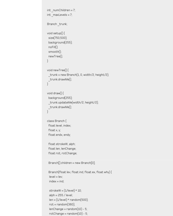
float strokeW, alph;
float len, lenChange;
float rot, rotChange;
You’ll need to initialize these properties, giving each level its own strokeWeight and alpha and each branch its own randomized set of length and rotation properties. Add this code before the line updateMe(ex, why); in the Branch constructor function:
strokeW = (1/level) * 100;
alph = 255 / level;
len = (1/level) * random(200);
rot = random(360);
lenChange = random(10) - 5;
rotChange = random(10) - 5;
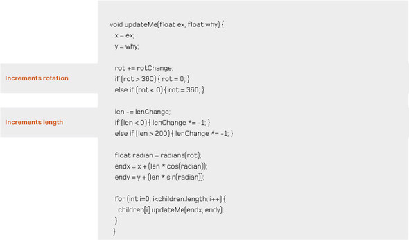
With these new properties, you can make the updateMe function actually do something when it’s called every frame. You’ll also give it the code to trickle down the command to its children so they can do something too, just as you did with the drawMe function. With this new version, the end point will be calculated according to the angle and length—plotting it as a point on the circumference of a circle of radius len. The angle to that point will change every frame, as will the length of the line. The new updateMe function is as follows.
Listing 8.2. updateMe that calculates the end point according to a rotating angle
You can update the object’s drawMe function to use the strokeW and alph properties you’ve defined and initialized. Also change the radius of the ellipse to be relative to the new variable length:
void drawMe() {
 strokeWeight(strokeW);
 stroke(0, alph);
 fill(255, alph);
 line(x, y, endx, endy);
 ellipse(endx, endy, len/12, len/12);
 for(int i=0; i<children.length; i++) {
   children[i].drawMe();
  }
}
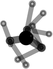
The final code is in listing 8.4 at the end of the next section, if you want to skip ahead. The output at this stage should look something like figure 8.5, except that in your version it will be spinning crazily like space clockwork. We’re purposely departing a little from the tree metaphor now. Every fractal programming tutorial I’ve ever read teaches you how to draw a tree and make it shake in the wind. But there are some things computers can do better than nature—one of which is space clockwork.
Figure 8.5. Space clockwork: the beginnings of an animated fractal, spinning like a dervish
Next, it’s time to turn it up to 11.
8.3. Exponential growth
Normally, the message at this point in the chapter would be to throw what you can at your structure and see what flies. But this time, let’s tread a little more cautiously. If you just start adding zeros to _numChildren and _maxLevels, things will seize up. Instead, try pushing up the numbers more gently. The following pages show images from _numChildren = 4; _maxLevels = 7; (figure 8.6) and _numChildren = 3; maxLevels = 10; (figure 8.7). Already this was nearing the point when my machine was starting to grumble. My amorphous blob was still spinning, but with a little less pizzazz.
Figure 8.6. Turning it up a little: four children, seven levels. I hope you’re coding along so you can see this structure moving.
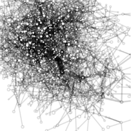
Figure 8.7. 3 children, 10 levels

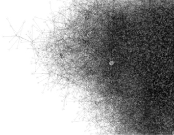
With a finer line (strokeW = (1/level) * 10;), you can get something that looks like figure 8.8. With this example I also added a conditional (if (level > 1)) to stop the drawMe function from drawing the trunk, which is clearly visible in figure 8.7.
Figure 8.8. A finer line, six levels, and seven children

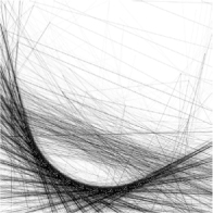
Figure 8.8 has six levels and seven children. Pushing that one further, to seven levels, yields something like figure 8.9. I found that was about the limit of what would still animate on my machine.
Figure 8.9. Seven children, seven levels: about as far as I could push it and expect it to animate
The complete code for this final version is in the following listing.
Listing 8.3. Final listing for the cog fractals

So far, we’ve looked at a single branching fractal structure, probably the simplest such system we might conceive. I’m not going to catalogue a long list of other possible shapes you could explore; I will leave the tinkering up to you. Instead, I’ll finish the chapter, and the book, with one specific example: a shape that was shown to me by a wise old mathematician on a dark and slightly overcast night—a shape that I’ve had a lot of fun with since.
8.4. Case study: Sutcliffe Pentagons
In 2008 I went to a meeting of the Computer Arts Society (CAS) in London, an organization that was (remarkably, for a body devoted to computing) celebrating its fortieth anniversary with that event. There, I heard a short talk by the society’s initiator and first chairman, the artist and mathematician Alan Sutcliffe.[1] Through this talk, he introduced me to a marvelous shape, which I have since mentally dubbed the Sutcliffe Pentagon.
1Alan has written about the early days of the CAS in the book White Heat Cold Logic: British Computer Art 1960–1980, Paul Brown, Charlie Gere, Nicholas Lambert, and Catherine Mason, editors (MIT Press, 2008).
To be clear, I’ve spoken to Alan about this, and he isn’t entirely over the moon with me using this name. He has been insistent that, even though he thought it up, he doesn’t believe the shape was his invention. He cites Kenneth Stephenson’s work on circle packing[2] as preceding him, in which Stephenson himself credits earlier work by Floyd, Cannon, and Parry.[3] But I have since reviewed this trail of influence, and, although Sutcliffe’s predecessors do describe a dissected pentagon, none of them take the idea half as far as he did. And even if they had, it wouldn’t change the way the Sutcliffe Pentagon was burned into my brain that particular evening.
2Kenneth Stephenson, Introduction to Circle Packing: The Theory of Discrete Analytic Functions (Cambridge University Press, 2005).
3J. W. Cannon, W. J. Floyd, and W. R. Parry, “Finite subdivision rules,” Conformal Geometry and Dynamics, vol. 5 (2001).
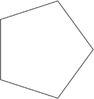
So, respecting Alan’s modesty, and his proviso that we probably shouldn’t, strictly speaking, refer to this construct as a Sutcliffe Pentagon, let me begin by showing you what a Sutcliffe Pentagon looks like (see figure 8.10). Then, I’ll talk you though how to construct a Sutcliffe Pentagon, and finally I’ll show you a number of different Sutcliffe Pentagon–derived works, developed using the Sutcliffe Pentagon structure.
Figure 8.10. Sutcliffe Pentagons

Sutcliffe noticed that if you draw a pentagon, then plot the midpoints of each of its five sides and extend a line perpendicular to each of these points, you can connect the end of these lines to make another pentagon. In doing this, the remaining area of the shape also ends up being subdivided into further pentagons, meaning that within each pentagon are six sub-pentagons. And within each of those, another six sub-pentagons, repeated downward toward the infinitesimal.
If you don’t find yourself overly thrilled by the mathematics of this yet, bear with me. In the following section, I’ll show what you can do with this simple principle. Let’s start by coding it up; then, I’ll demonstrate some of the directions I took it in.
8.4.1. Construction
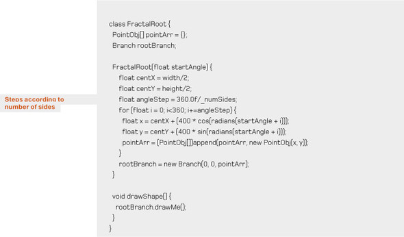
You begin by drawing a regular pentagon. But the way I approached it, you don’t just draw five lines between five points; instead, you create a drawing method that is a little more generic—rotating 360 degrees around a center and extrapolating points at certain angles. For example, if you plot a point every 72 degrees, you get a pentagon.
Listing 8.4. Drawing a pentagon using rotation
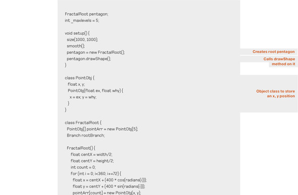

The FractalRoot object contains an array of five points. It fills that array by rotating an angle around a center point in 72-degree jumps. It then uses that array of points to construct the first Branch object. The Branch object is your self-replicating fractal object. Each branch draws itself by connecting the points it has placed in its outerPoints array.
This should give you a pentagon, as shown in figure 8.11.
Figure 8.11. Just in case you don’t know what a regular pentagon looks like
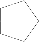
Next, you plot the midpoints of each side. Add the two functions in the following listing to the Branch object.
Listing 8.5. Functions to calculate the midpoints of a set of vertices
PointObj[] calcMidPoints() {
  PointObj[] mpArray = new PointObj[outerPoints.length];
  for (int i = 0; i < outerPoints.length; i++) {
   int nexti = i+1;
   if (nexti == outerPoints.length) { nexti = 0; }
   PointObj thisMP = calcMidPoint(outerPoints[i], outerPoints[nexti]);
  mpArray[i] = thisMP;
 }
 return mpArray;
 }

 PointObj calcMidPoint(PointObj end1, PointObj end2) {
  float mx, my;
  if (end1.x > end2.x) {
    mx = end2.x + ((end1.x - end2.x)/2);
   } else {
    mx = end1.x + ((end2.x - end1.x)/2);
   }
   if (end1.y > end2.y) {
     my = end2.y + ((end1.y - end2.y)/2);
   } else {
    my = end1.y + ((end2.y - end1.y)/2);
   }
   return new PointObj(mx, my);
 }
The first function, calcMidPoints, iterates through the array of outer points and passes each pair of points to the second function, calcMidPoint; this function works out the difference between each individual pair, covering every possible relative position to each other. calcMidPoints collects each of the results in an array to pass back.
You call the new function in the Branch constructor and put the result in an array named midpoints:
PointObj[] midPoints = {};

Branch(int lev, int n, PointObj[] points) {
  ...

  midPoints = calcMidPoints();
}
Then, you can plot those points in the drawMe function:
strokeWeight(0.5);
fill(255, 150);
for (int j = 0; j < midPoints.length; j++) {
 ellipse(midPoints[j].x, midPoints[j].y, 15, 15);
}
This gives you figure 8.12.
Figure 8.12. Calculating the midpoints of the sides
The next set of points you need are the ends of the struts to extend from the midpoints. You don’t need to work this out relative to the angle of the side vertex; you can instead use one of the opposite points of the shape to aim toward.
First, define a global _strutFactor variable to specify the ratio of the total span you want the strut to extrude:
float _strutFactor = 0.2;
Now, the Branch object needs another set of functions to plot those points.
Listing 8.6. Functions to extend the midpoints toward the opposite points


Again, add this code to the Branch constructor:
PointObj[] projPoints = {};

Branch(int lev, int n, PointObj[] points) {

...
  projPoints = calcStrutPoints();
}
And plot those points in the drawMe function so you can see they’re correct:
strokeWeight(0.5);
fill(255, 150);
for (int j = 0; j < midPoints.length; j++) {
 ellipse(midPoints[j].x, midPoints[j].y, 15, 15);
 line(midPoints[j].x, midPoints[j].y, projPoints[j].x, projPoints[j].y);
 ellipse(projPoints[j].x, projPoints[j].y, 15, 15);
}
You should be looking at something like figure 8.13.
Figure 8.13. Project struts toward the opposite points

Now you have all the points you need for the recursive structure. You can test this first by passing the five strut points as the outer points for an inner pentagon. Add the following to the Branch object’s constructor:
Branch[] myBranches = {};

Branch(int lev, int n, Point[] points) {

  ...
  if ((level+1) < _maxlevels) {
   Branch childBranch = new Branch(level+1, 0, projPoints);
   myBranches = (Branch[])append(myBranches, childBranch);
  }
}
Then, add a similar trickle-down method to the drawMe function so the children are rendered to the screen:
void drawMe() {

...
  for(int k = 0; k < myBranches.length; k++) {
     myBranches[k].drawMe();
  }
}
You should see the result shown in figure 8.14.
Figure 8.14. A recursive pentagon
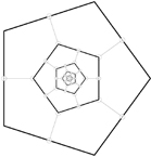
Adding the other five pentagons to create a complete Sutcliffe Pentagon fractal is just a matter of passing the points to five more new Branch objects. The code is as follows:
if ((level+1) < _maxlevels) {

  ...
  for (int k = 0; k < outerPoints.length; k++) {
   int nextk = k-1;
   if (nextk < 0) { nextk += outerPoints.length; }
   PointObj[] newPoints = {  projPoints[k], midPoints[k],
           outerPoints[k], midPoints[nextk], projPoints[nextk] };
   childBranch = new Branch(level+1, k+1, newPoints);
   myBranches = (Branch[])append(myBranches, childBranch);
  }
}
This gives you the fractal shown at the beginning of this section in figure 8.10. Now you can begin experimenting with it.
8.4.2. Exploration
You have the ratio of the projected strut in a handy variable, so let’s start by varying this. You’ll add a draw loop to redraw the fractal every frame with a new strut length, and vary that length by a noise factor. For this modification, you don’t need to do anything to the objects—just update the initialization section of the code as shown in the following listing.
Listing 8.7. Varying the strut length of a Sutcliffe Pentagon
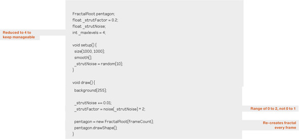
You make one other little change here: you pass the frameCount to the FractalRoot object. If you then modify FractalRoot, you can use that number to increment the angle and make the shape spin, Space Odyssey style:
FractalRoot(float startAngle) {
...
    float x = centX + (400 * cos(radians(startAngle + i)));
    float y = centY + (400 * sin(radians(startAngle + i)));
...
}
Also notice that the strut ratio doesn’t just vary between 0 and 1, we’ve allowed it to go to 2, so it can extend beyond the limits of the shape. Does this work? Try it and see. How about if the strut ratio went into negative values? What would happen then? Only one way to find out:
_strutFactor = (noise(_strutNoise) * 3) - 1;
In this case, the ratio varies between -1 and +2. You end up with an animation that produces shapes like those shown in figure 8.15.
Figure 8.15. Strut factors -1 through to +2
Already it’s getting interesting.
Although the pentagon has a neat symmetry, there is no reason why your starting shape has to have five sides. One of the reasons I adopted the non-absolute method of drawing the pentagon was that it made it easy to add extra sides to the polygon. For example, create a global variable:
int _numSides = 8;
Now, change the FractalRoot class as shown in this listing.
Listing 8.8. Sutcliffe Pentagon, not limited to five sides
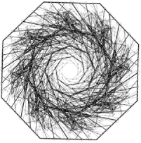
Now you have a structure capable of handling any number of sides. How about eight, as shown in figure 8.16?
Figure 8.16. Eight sides: a Sutcliffe Octagon?
Or 32? (See figure 8.17.)
Figure 8.17. A 32-sided structure
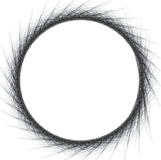
Taking another approach, why should you feel limited to 360 degrees? I discovered that setting the angle step to 133 and stepping 8 times (effectively turning the circle three times) gave me something like figure 8.18.
Figure 8.18. Angle step of 133, through 1024 degrees

I followed this line of exploration by making the angles and the number of sides vary according to a noise factor between frames, in the same way you varied the strut factor. You shouldn’t have any difficulty working out the code if you want to try it. Through this process, I discovered what an incomplete revolution looks like (see figure 8.19).
Figure 8.19. The system is resilient enough to work with irregular and incomplete shapes.
The fractal structure I built (to Sutcliffe’s specification) proved to be extremely mathematically sturdy, as long as I didn’t turn the number of levels up too high. This meant I could wrench it about as if I were throttling a ferret, with the only consequence being that the results became less linear and more interesting.
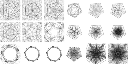
I hope you’re beginning to appreciate why this single fractal delighted me so when I started playing with it. Figure 8.20 shows a few of the ideas I’ve tried. You can find the code for all of these, along with the finished code for this section, at http://abandonedart.org.
Figure 8.20. A number of abandonedart.org applications of the Sutcliffe Pentagon

This is where we leave fractals—and where we leave the book, too. If you can get your head around the code in this chapter, there really is nothing you can’t conquer in Processing.
8.5. Summary
Fractals, another organizational structure we’ve stolen from the natural world, share a similar principle to the emergent structures we experimented with in earlier chapters. Simple code can produce complex results when magnified through reflexive recursion.
The main themes of this book have been unpredictability, emergent complexity, and fresh approaches to programming. In part 1, I introduced generative art, the Processing language and IDE, and the idea of allowing a certain artistic flourish into the strict discipline of programming. In part 2, our focus was on ways to force our computers into surprising us with unexpectedly sophisticated aesthetics, using random functions, noise functions, and mathematical constructions that produced results beyond what we can work out in our heads.
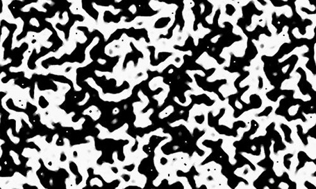
In this final part, the unpredictability we fostered arose from emergence; the interplay between large numbers of simple elements giving rise to levels of complexity beyond the competence of our humble programming skills. The manipulations of logic and procedure that we perform when creating generative art, no matter how abstract, clearly share principles with the more sophisticated computations of the natural world. Craig Reynold’s Boids (chapter 6) performs a pretty good imitation of murmating starlings; two-state cellular automata produce patterns that are equally familiar to sociologists, biologists, and geologists (see figure 8.21 and chapter 7). Recursive fractal constructions are at their root an idea stolen from natural organization, as you’ve seen in this chapter.
Figure 8.21. Patterns generated using the Vicniac Vote rule from chapter 7
Despite how it may look when viewed through a screen, we don’t live in a digital world. Our reality is stubbornly analog: it doesn’t fit into distinctly encodable states. It’s an intricate, gnarly, and indefinite place. If we want to use digital tools to create art, which somehow has to reflect our crazy, chaotic existence, we need to allow imperfection and unpredictability into the equation. But, as I hope I’ve shown, there is room for the organic within the mechanical, and programming isn’t just about efficiency and order. Our computing machines, which may only be capable of producing poor imitations of life, are tapping a computational universality that the natural world shares.
Programming generative art, if I were to try and sum up it up into a single pocket-sized nugget, is about allowing the chaos in. Not all things in life benefit from a structured approach; there is much that is better for a little chaotic drift. If you have a way of working that allows this freedom, permitting inspiration to buffet you from idea to idea, you’ll inevitably end up in some interesting places.
Thanks for reading.
Note: If you found value in this book and want to share it with a friend (and I’d appreciate it if you did), the Creative Commons chapters are free to distribute. You can download them from http://zenbullets.com.