Chapter 11. Patterns in functional programming

 

 

Functional programming is the practice of composing programs using functions. It’s an area of software design and architecture that has been neglected in mainstream books and classes since the emergence of object-oriented programming. Functional programming offers a lot to the object-oriented developer and can nicely complement standard object-oriented practices.

Functional programming is a relatively large topic to try to compress into a single chapter. Instead, this chapter introduces a few key abstractions used in functional programming and demonstrates their usage in two different situations. The goal is to show one of the many styles of functional programming, rather than turn you into an expert functional programmer.

First, a discussion on some fundamental concepts behind the patterns in functional programming.

11.1. Category theory for computer science

Category theory is the mathematical study of collections of concepts and arrows. For the purposes of computer science, a concept is a type, like String, Int, and so on. An arrow is a morphism between concepts—something that converts from one concept to another. Usually in computer science, a morphism is a function defined against two types. A category is a grouping of concepts and arrows. For example, the category of cats includes all the various types of cats in the world as well as the captions needed to convert from a serious cat into a lol cat. Category theory is the study of categories like these and relationships between them. The most used category in programming is the categories of types: the classes, traits, aliases and object self types defined in your program.

Category theory shows up in many corners of programming but may not always be recognized. This section will introduce a library to configure software and introduce the concepts from category theory that are used in the library.

A good way to think of category theory, applied to functional programming, is design patterns. Category theory defines a few low-level abstract concepts. These concepts can be directly expressed in a functional language like Scala and have library support. When designing software, if a particular entity fits one of these concepts, a whole slew of operations immediately becomes available as well as the means to reason through usage. Let’s look at this concept in the context of designing a configuration library.

In section 2.4 we explored the usage of Scala’s Option class as a replacement for nullable values. In particular, this section showed how we can use Options to create walled gardens—that is, functions can be written as if all types aren’t null. These functions can be lifted into functions that will propagate empty values. Let’s look at the lift3 function from chapter 2:

scala>   def lift3[A,B,C,D](f: Function3[A,B,C,D]) = {
     |     (oa: Option[A], ob: Option[B], oc: Option[C]) =>
     |        for(a <- oa; b <- ob; c <- oc) yield f(a,b,c)
     |   }
lift3: [A,B,C,D](f: (A, B, C) => D)(
  Option[A], Option[B], Option[C]) => Option[D]

The lift3 function takes a function defined against raw types and converts it to a function that works with Option types. This lets us wrap Java’s DriverManager.getConnection method directly and make it option-safe.

The lift3 function uses Scala’s for expression syntax. Scala’s for expressions are syntactic sugar for the map, flatMap, foreach, and withFilter operations defined on a class. The for expression

for(a <- oa; b <- ob; c <- oc) yield f(a,b,c)

is desugared into the following expression:

oa.flatMap(a => ob.flatMap(b => oc.map(c => f(a,b,c))))

Each <- of the for expression is converted into a map or flatMap call. These methods are each associated with a concept in category theory. The map method is associated with functors, and the flatMap method is associated with monads. For expressions make an excellent way to define workflows, which we define in section 11.4.

A monad is something that can be flattened. Option is a monad because it has both a flatten and flatMap operation that abide by the monadic laws. We’ll cover the details of monads in section 11.2.2. For now, let’s first generalize the advanced Option techniques from section 2.4.1.

Imagine that we’re designing a configuration library. The goal is to use this library, in combination with a variant of the lift3 method, to construct database connections based on the current configuration parameters. This library could read configuration parameters from different locations. If any of these locations are updated, the program should automatically alter its behavior the next time a database connection is requested. Let’s define a new trait, Config, that will wrap this logic for us. Because the filesystem is volatile and configuration isn’t guaranteed to exist, the Config library will also make use of the Option trait to represent configuration values that weren’t found. Let’s define a minimal Config trait.

trait Config[+A] {
  def map[B](f : A => B) : Config[B]
  def flatMap[B](f : A => Config[B]): : Config[B]
  def get : A
}

The Config trait consists of three methods. The first, map, takes a function that operates on the data stored in the Config object and returns a new Config object. This is used to transform the underlying configuration data. For example, when reading environment variables of strings, the map method could be used to convert an environment variable into an Integer.

The next method is flatMap. This method takes a function against the current Config object and returns a second Config object. You can use this to construct new Config objects based on values stored in an initial Config object. For example, imagine we have a Config[java.io.File] that holds the location of a secondary configuration file. We can use the flatMap operation to read this location and then extract more configuration values from that location.

The final method is called get. This method is unsafe, in that it will attempt to read the current configuration environment, wherever configuration is defined to be, and return the resulting configuration values. As with Option, you shouldn’t use this method until the code calling it knows what to do in the event of failure. Also, because the get method will read the environment, it can be expensive if performed within a tight loop of the software.

Let’s define a construction operation for Config. Creating a new Config object is the case of defining the get method, because map and flatMap can be implemented in terms of get. For now, let’s assume that map and flatMap are implemented appropriately (see the source code for implementations).

object Config {
  def apply[A](data : => A) = new Config[A] {
    def get = data
  }
}

The Config object defines a single method called apply, which is the constructor for Config objects. The apply method takes one parameter, a by-name parameter. By-name parameters in Scala are similar to no-argument functions in that they’ll evaluate their associated expressions every time they’re referenced. This means that defining the get method to reference the data argument will cause the data parameter to be reevaluated each time it’s referenced. Here’s an example:

scala> var x = 1
x: Int = 1

scala> Config({ x += 1; x})
res2: java.lang.Object with config.Config[Int] = ...

scala> res2.get
res3: Int = 2

scala> res2.get
res4: Int = 3

First, the variable x is defined as equal to 1. Next, a Config object is constructed. The argument is the expression { x +=1; x}. This expression should be evaluated every time the Config’s get method is called. The next line calls the get method, and the returned value is 2. The next line calls the get method again and the return value is now 3. Let’s create a few convenience methods to read configuration locations.

def environment(name : String) : Config[Option[String]] =
    Config(if (System.getenv.containsKey(name))
      Some(System.getenv.get(name))
    else None)

The environment method will read configuration values from the process environment. The method takes a string of the environment variable to read. The Config object is constructed using an if expression. If the environment variable is available, the value is returned inside an Option. If the variable isn’t available, a None is returned. The full type returned is a Config[Option[String]]. Let’s try this out on the command line:

> export test_prop="test_prop"
> scala -cp .
...
scala> val test = environment("test_prop")
test: Config[String] = Config$$anon$1@659c2931

scala> test.get
res0: String = test_prop

First, the environment variable test_prop is exported. Next, the Scala REPL is started and a Config object pointing to the test_prop property value is created. When calling get on this test property, the correct value is displayed.

Now let’s look into constructing database connections based on environment variables. Here’s the original code from section 2.4:

scala>   def lift3[A,B,C,D](f : Function3[A,B,C,D]) = {
     |     (oa : Option[A], ob : Option[B], oc : Option[C]) =>
     |        for(a <- oa; b <- ob; c <- oc) yield f(a,b,c)
     |   }
lift3: [A,B,C,D](f: (A, B, C) => D)(
  Option[A], Option[B], Option[C]) => Option[D]

scala> lift3(DriverManager.getConnection)

The lift3 method takes a three-argument function and converts it into a three-argument function that works against Option arguments. This is used on the Driver-Manager.getConnection method to construct a new method that operates on Options.

Using DriverManager with the new Config library requires lifting the getConnection function to take Config[Option[String]] rather than just Option[String]. Let’s take the simple approach of defining a new lift function to convert three-argument methods into methods that operate on Config objects.

def lift3Config[A,B,C,D](f : Function3[A,B,C,D]) = {
  (ca : Config[A], cb : Config[B], cc : Config[C]) =>
     for(a <- ca; b <- cb; c <- cc) yield f(a,b,c)
}

The lift3Config method takes a three-argument function as its own argument. It returns a new function that takes Config traits of the original parameters. The implementation uses for expressions to call the underlying flatMap and map operations on the Config object. The final result is a Config object wrapping the underlying data. Let’s use this to define a DatabaseConnection that uses environment variables.

scala> val databaseConnection =
     |  lift3Config(DriverManager.getConnection)(
     |   Config.environment("jdbc_url"),
     |   Config.environment("jdbc_user"),
     |   Config.environment("jdbc_password"))
databaseConnection: Config[java.sql.Connection]

The lift3Config method is called against the lift3 method called on DriveManager.getConnection. This creates a three-argument function that works on Config[Option[String]] types. Finally, this new function is passed three arguments, one for each environment variable. The resulting Config object will construct a new database connection if the environment variables jdbc_url, jdbc_user, and jdbc_password are all available.

This implementation of lift3Config should look familiar. It’s almost identical to the lift3 method because both the Config trait and the Option trait are instances of the same abstract concept from category theory. Let’s try to reverse engineer the raw concepts behind the lift method to see if we can rescue it for both Option and Config.

11.2. Functors and monads, and how they relate to categories

Functors are transformations from one category to another that can also transform and preserve morphisms. A morphism is the changing of one value in a category to another in the same category. In the example of the category of cats, a morphism would be akin to a box that takes a dim cat and converts it into a neon glowing cat. In the category of types, the most commonly used in computer science, a morphism is a function that converts from one type to another. The functor would be something that converts cats into dogs. The functor would be able to convert dim cats into dim dogs and glowing cats into glowing dogs. The functor could also convert the box so that it can convert dim dogs into glowing dogs.

Figure 11.1 illustrates functors.

Figure 11.1. Functor transforming types and functions

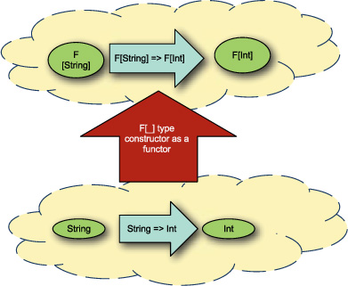
The circle on the bottom represents the category of all possible types. Inside are the standard String, Double, Int, and any other type that can be defined in Scala. The functor F is a type constructor in Scala. For any type T that’s in the category on the bottom, you can place that type in the type constructor F[_] and get a new type F[T] shown on the top category. For example, for any type T, a Config[T] can be made. The Config class is a functor.

 

Laws of Functors and Other Properties

Functors, and the other concepts described in this chapter, have mathematical laws that govern their behavior. These laws provide a default set of unit tests as well as standard transformations that can be performed on code. This book doesn’t cover the laws in detail, but we give sufficient grounding in Category theory for you to investigate these laws as needed.

 

For the transformation to be a functor transformation, it means that all morphisms must be preserved in the transformation. If we have a function that manipulates types in the first category, we should have a transformed function that operates on the transformed types. For example, if I have a function that takes a String and converts it to an Int, I should be able to also take a Config[String] instance and convert it to a Config[Int] instance. This is what the map method on Option and Config grant. Let’s convert this into an interface:

Listing 11.1. Functor typeclass

trait Functor[T[_]] {
   def apply[A](x: A): T[A]
   def map[A,B](x : T[A])(f: A=>B) : T[B]
}

The apply method grants the first property of functors. For any type A, a Functor can construct a type T[A] in the new category. The map method grants the second property of functors. Given a transformed type T[A] and a morphism in the original category A=>B, a value T[B] can be created. We have a new function that takes T[A] and returns T[B].

Let’s implement the Functor interface for Config.

object ConfigAsFunctor extends Functor[Config] {
  def apply[A](x : A): Config[A] = Config(x)
  def map[A,B](x : Config[A])(f: A=>B) = x.map(f)
}

The Functor implementation for Config is defined such that the apply method calls the Config companion object’s apply method. The map method can delegate to the underlying map method on the Config class.

Finally, let’s create a bit of syntactic sugar so that the map method on the Functor typeclass appears to be on the raw type.

implicit def functorOps[F[_] : Functor, A](ma: F[A]) = new {
  val functor = implicitly[Functor[F]]
  final def map[B](f: A => B): F[B] = functor.map(ma)(f)
}

The implicit method functorOps creates a new anonymous class that has a local map method that accepts only a function A => B. This simplifies the remaining code samples using Functor.

Now, we’ll create the lift method so that it’s generic against the Functor abstraction.

def lift[F[_] : Functor] = new {
   val functor = implicitly[Functor[F]]
   def apply3[A,B,C,D](f: (A,B,C) => D): (
     F[A],F[B],F[C]) => F[F[F[[D]]] = {
       (fa, fb, fc) =>
          fa map { a =>
            fb map { b =>
              fc map { c =>
               f(a,b,c)
              }
            }
          }
   }
}

The new lift method uses a Functor to promote elements of the function. The apply3 method accepts a three-argument function and calls map against each of these methods to chain the method calls. The resulting function is one that accepts all the original arguments inside the FunctorF[_] and returns a nested result type F[F[F[D]].

The issue with this method is that the resulting type is F[F[F[D]]], not F[D]. This means for the config library, creating a database connection will result in a Config[Config[Config[Connection]]] instead of a Config[Connection]. To resolve this, let’s create a new type trait the extends Functor and adds a flatten method. This method will be responsible for collapsing the pattern F[F[D]] to F[D], which should allow the above function to work as desired. This new trait is called a Monad.

11.2.1. Monads

Monads are a means of combining a functor application, if that functor is an endofunctor. An endofunctor is a functor that converts concepts and morphisms in its category back into the same category. Using the cat example, an endofunctor would be a way of converting cats and genetic cat manipulations into different types of cats and cat genetic manipulations. Transforming a cat more than once by the same functor could be reduced into single functor application. Similarly, altering cat genetic manipulations more than once can be reduced into a single alteration.

In computer science, monads are often used to represent computations. A monad can be used to abstract out the execution behavior of a program. Some monads can be used to handle concurrency, exceptions, or even side effects. Using monads in workflows or pipelines is discussed in section 11.4.

Let’s look at the programming definition of a monad in the following listing:

Listing 11.2. Monad typeclass

trait Monad[T[_]] {
  def flatten[A](m : T[T[A]]): T[A]
  def flatMap[A,B](x : T[A])(f : A => T[B]
    )(implicit func: Functor[T]): T[B] =
      flatten(func.map(x, f))
}

The Monad trait defines the flatten and flatMap methods. The flatten method is used to take a double wrapped type and turn it into a wrapped type. If a Functor T[_] is applied twice, the monad knows how to combine this to one application. For example, the List monad can convert a list of lists into a single list with all the underlying elements of the nested lists. The Monad trait also provides a convenience function flatMap, which chains the flatten and map calls for convenience.

 

 

Monads are, among other things, a means of preventing bloat in types and accessors. We can take a nested list of lists and treat it as a single list, which has a more convenient syntax.

Again, let’s create a convenience implicit to reduce the syntactic noise of using the Monad type trait.

implicit def monadOps[M[_] : Functor : Monad, A](ma: M[A]) = new {
  val monad = implicitly[Monad[M]]
  def flatten[B](implicit $ev0: M[A] <:< M[M[B]]): M[B] =
    monad.flatten(ma)
  def flatMap[B](f: A => M[B]): M[B] =
    monad.flatMap(ma)(f)
}

The implicit method monadOps creates a single anonymous class. The flatten method uses the implicit type constraint trick from section 7.2.3 to ensure that the value inside the monad M[_] is another M[_] value. The flatMap method delegates to the Monad trait’s flatMap method.

Now, let’s modify the lift function to make use of the Monad trait.

def lift[F[_] : Monad : Functor] = new {
   val m = implicitly[Monad[F]]
   val func = implicitly[Functor[F]]
   def apply3[A,B,C,D](f: (A,B,C) => D): (F[A], F[B], F[C]) => F[D] = {
        (fa, fb, fc) =>
          m.flatMap(fa) { a =>
            m.flatMap(fb) { b =>
              func.map(fc) { c =>
               f(a,b,c)
              }
            }
          }
   }
}

The new lift method uses a Monad type class instead of a Functor. This lift method looks similar to the original lift method for Option, except that it can generically lift functions to operate against monads. Let’s try it out.

scala> lift[Option] apply3 java.sql.DriverManager.getConnection
res4: (Option[String], Option[String],
       Option[String]) => Option[java.sql.Connection] =
    <function3>

The lift method is called using Option as the type parameter. The apply3 method is called directly against java.sql.DriverManager.getConnection(...). The result is a new function that accepts three Option[String] values and returns an Option[Connection].

Monads and functors form the basic building blocks of lots of fundamental concepts in programming. We’ll explore these more in depth in section 11.4. An abstraction lives between monads and functors. This abstraction can be used as an alternative mechanism of writing the lift function. Instead of relying on a flatMap operation, a function can curried and values fed into it in an applicative style.

11.3. Currying and applicative style

Currying is the conversion of a function of multiple parameters into a chain of functions that accept a single parameter. A curried function accepts one of its arguments and returns a function that accepts the next argument. This chain continues until the last function returns a result. In Scala, any function of multiple parameters can be curried.

Applicative style refers to using curried functions to drive parameters in applicative functors through them. Applicative functors are functors that also support a method to convert mapped morphisms into morphisms against mapped types. In English, this means that if we have a list of functions, an applicative functor can create a single function that accepts a list of argument values and returns a new list of results.

11.3.1. Currying

Currying is taking a function of several arguments and turning it into a function that takes a single argument and returns a function that takes the next argument that returns a function that takes the next argument and so on, until finally one of the functions returns a value. In Scala, all functions have a curried method that can be used to convert them from multiargument functions into curried functions. Let’s try it out:

scala> val x = (x:Int, y:Double, z: String) => z+y+x
x: (Int, Double, String) => java.lang.String = <function3>

scala> x.curried
res0: (Int) => (Double) => (String) => java.lang.String = <function1>

The first line constructs a function that takes three arguments: an integer, a double, and a string. The second calls curried against it, which returns a function of the type Int => Double => String => String. This function takes an Int and returns another function Double => String => String. This function takes a Double and returns a function that takes a String and returns a String. A single function of multiple arguments is converted into a chain of functions, each returning another function until all arguments have been satisfied and a return value is made. Currying is pretty easy to do by hand; let’s try it out.

scala> val y = (a: Int) => (b: Double) => (c: String) => x(a,b,c)
y: (Int) => (Double) => (String) => java.lang.String = <function1>

This line constructs an anonymous function y that takes an Int, called a, and returns the function defined by the rest of the expression. This same trick defines a nested anonymous function, until eventually the function x defined earlier is called. Note that this function has the same signature as x.curried. The trick is that each call to a function captures a portion of the argument list of the original function and returns a new function for the remaining values.

This trick can be used when attempting to promote a function of multiple simple parameters to work with values inside a Functor. Let’s redefine the lift method to use only a Functor.

def lift[F[_]: Functor] = new {
   def apply3[A,B,C,D](f: (A,B,C) => D): (F[A], F[B], F[C]) => F[D] = {
       (fa, fb, fc) =>
          val tmp: F[B => C => D] = fa.map(f.curried)
          ...?...
   }
}

The new implementation for the apply3 method in lift uses the map operation on Functor against the curried function. The result is a function B => C => D wrapped inside the F[_] functor.

Let’s break this down to see what’s happening in the types. First a curried function is created.

scala> f.curried
res0: A => (B => C => D) = <function1>

The parentheses in the resulting expression have been adjusted to show the true type. The result is a single function that takes an A and produces a value. Because the fa parameter is a value of F[A], we can combine the curried function with the fa value using the map method.

scala> fa.map[B => C => D](f.curried)
res0: F[B => (C => D)] = Config(<function1>)

The map method on fa is called against the curried function. The result is a F[_] containing the rest of the function. Remember the Functor defines its map method as def map[A,B](m: F[A])(f: A=> B): F[B]. In this case the second type parameter is a function B=>C=>D.

Now there’s a problem. The code can’t continue to use the map method defined on Functor because the remaining function is wrapped inside the functor F[_]. To solve this, let’s define a new abstraction, Applicative, as shown in the following listing:

Listing 11.3. Applicative typeclass

trait Applicative[F[_]] {
  def lift2[A,B](f: F[A=>B])(ma: F[A]): F[B]
}

The Applicative trait is defined for the type F[_]. It consists of one method, lift2, that takes a function inside an F[_] and a value inside an F[_] and returns the result inside an F[_]. Notice that this is different from a monad, which can flatten F[F[_]]. The lift method can now be completed using applicative functors.

def lift[F[_]: Functor: Applicative] = new {
    val func = implicitly[Functor[F]]
    val app = implicitly[Applicative[F]]
    def apply3[A,B,C,D](f: (A,B,C) => D): (F[A], F[B], F[C]) => F[D] = {
       (fa, fb, fc) =>
          val tmp: F[B => C => D] = func.map(fa)(f.curried)
          val tmp2: F[C => D] = app.lift2(tmp)(fb)
          app.lift2(tmp2)(fc)
    }
  }

The lift function now requires both a Functor and an Applicative context bound. As before, the function is curried and applied against the first argument using the functor’s map method. But the applicative functor’s lift2 method can be used to apply the second argument of the function. Finally, the lift2 method is used again to apply the third argument of the original function. The final result is the value of type D wrapped inside the functor F[_].

Now, let’s try the method against the previous example of using the Driver-Manager.getConnection method.

scala> lift[Config] apply3 java.sql.DriverManager.getConnection
res0: (Config[String], Config[String],
       Config[String]) => Config[java.sql.Connection] =
    <function3>

The result is the same as it was for using functor and monad. The two reasons to choose this style instead is that there are more things that can implement the lift2 method for applicative functors than can implement the flatten method for monads and that applicative functors can compute in parallel while monadic workflows are sequential.

11.3.2. Applicative style

An alternative syntax to lifting functions into applicative functors is known as applicative style. This can be used in Scala to simplify the construction of complex function dependencies, keeping the values inside an applicative functor. For example, using the Config library defined earlier, you can construct an entire program from functions and applicative applications. Let’s take a look.

 

 

Assuming there’s a software system that’s composed of two subsystems: the DataStore and the WorkerPool. The class hierarchy for this system looks as follows:

trait DataStore { ... }
trait WorkerPool { ... }
class Application(ds: DataStore, pool: WorkerPool) { ... }

The DataStore class and WorkerPool class are defined with all the methods required for their subcomponent. The Application class is defined as taking a DataStore instance and a WorkerPool instance. Now, when constructing the application, the following can be done with applicative style:

def dataStore: Config[DataStore]
def workerPool: Config[WorkerPool]
def system: Config[Application] =
  (Applicative build dataStore).and(
   workerPool) apply (new Application(_,_))

The dataStore and workerPool methods are defined as abstraction constructors of DataStore inside a Config object. The entire system is composed by creating an Applicative instance on the dataStore, combining the workerPool and applying that to an anonymous function (new Application(_,_)). The result is an Application embedded in a Config object. The Applicative call creates a builder that will use the Config[_] instances to construct something that can accept a function of raw types and return a resulting Config object.

 

Haskell Versus Scala

Applicative style came to Scala from the Haskell language, where functions are curried by default. The syntax presented here is a Scala idiom and doesn’t mimic the Haskell directly. In Haskell, applicative style uses the <*> operator, called apply, against a curried function on Applicative functors—that is, Haskell has a <*> method that performs the same function as the lift2 method in the Applicative trait.

 

This applicative style, combined with the Config class, can be used to do a form of dependency injection in Scala. Software can be composed of simple classes that take their dependencies in the constructor and a separate configuration can be used to wire all the pieces together using functions. This is an ideal blend of object orientation and functional programming in Scala. For example, if the DataStore trait had an implementation that used a single JDBC connection like the following:

class ConnectionDataStore(conn: java.sql.Connection) extends DataStore

Then the entire application can be configured as shown in the following listing:

Listing 11.4. Configuring an application using the Config class and applicative builder

def jdbcUrl: Config[String] = environment("jdbc.url")
def jdbcUser: Config[String] = environment("jdbc.user")
def jdbcPw: Config[String] = environment("jdbc.pw")
def connection: Config[Connection] =
  (Applicative build jdbcUrl).and(jdbcUser).and(jdbcPw).apply(
    DriverManager.getConnection)

def dataStore: Config[DataStore] =
  connection map (c => new ConnectionDataStore(f))
def workerPool: Config[WorkerPool] = ...

def system: Config[Application] =
  Applicative build dataStore and workerPool apply (
    new Application(_,_))

The environment function is defined in 11.7. This function pulls the value of an environment variable if it exists and is used to pull values for the JDBC connection’s URL, user, and password. The applicative builder is then used to construct a Config [Connection] using these config values and the DriverManager.getConnection method directly. This connection is then used to construct the dataStore configuration using the map method on Config to take the configured JDBC connection and use it to instantiate the ConnectionDataStore. Finally, the applicative builder is used to construct the application from the dataStore and workerPool configuration.

Although this is pure Scala code, the concept should look familiar to users of Java inversion-of-control containers. This bit of code represents the configuration of software separate from the definition of its components. There’s no need to resort to XML or configuration files in Scala.

Let’s look at how the Applicative object build method works.

object Applicative {
  def build[F[_]: Functor: Applicative, A](m: F[A]) =
    new ApplicativeBuilder[F,A](m)
}

The build method on Applicative takes two types, F[_] and A. The F[_] type is required to have an applicative and functor instance available implicitly. The build method accepts a parameter of type F[A] and returns a new ApplicativeBuilder class. Let’s look at the ApplicativeBuilder class in the following listing:

Listing 11.5. ApplicativeBuilder class

class ApplicativeBuilder[F[_],A](ma: F[A])(
    implicit functor: Functor[F], ap: Applicative[F]) {
  import Implicits._

  def apply[B](f: A => B): F[B] = ma.map(f)

  def and[B](mb: F[B]) = new ApplicativeBuilder2(mb)
  class ApplicativeBuilder2[B](mb: F[B]) {

    def apply[C](f: (A, B) => C): F[C] =
      ap.lift2((ma.map(f.curried)))(mb)

    def and[C](mc: F[C]) = new AppplicativeBuilder3[C](mc)

    class AppplicativeBuilder3[C](mc: F[C]) {

      def apply[D](f: (A,B,C) => D): F[D] =
        ap.lift2(ap.lift2((ma.map(f.curried)))(mb))(mc)

      ...
    }
  }
}

The ApplicativeBuilder class takes in its constructor the same arguments as the Applicative.build method. The class consists of two methods, apply and and, as well as a nested class ApplicativeBuilder2. The apply method takes a function against raw types A and B and applies the captured member ma against it, creating an F[B]. The and method takes another applicative functor instance of type F[B] and constructs an ApplicativeBuilder2. The ApplicativeBuilder2 class also has two methods: apply and and. The apply method is a bit more odd. Like the lift example earlier, this method curries the raw function f and uses the map and lift2 methods to feed arguments to the lifted function inside the functor. The and method constructs an ApplicativeBuilder3 that looks a lot like ApplicativeBuilder2 but with one more parameter. This chain of nested builder classes goes all the way to Scala’s limit on anonymous function arguments of 23.

Applicative style is a general concept that can be applied in many situations. For example, let’s use it to compute all the possible pairings of elements from two collections.

scala> (Applicative build Traversable(1,2) and
    Traversable(3,4) apply (_ -> _))
res1: Traversable[(Int, Int)] =
    List((1,3), (1,4), (2,3), (2,4))

The Applicative builder is used to combine two Traversable lists. The apply method is given a function that takes two arguments and creates a pairing of the two. The resulting list is each element of the first list paired with each element of the second list.

Functors and monads help express programs through functions and function transformations. This applicative style, blended with solid object-oriented techniques, leads to powerful results. As seen from the config library, applicative style can be used to blend pure functions and those that wall off dangers into things like Option or Config. Applicative style is usually used at the interface between raw types like String and wrapped types like Option[String].

Another common use case in functional programming is creating reusable workflows.

11.4. Monads as workflows

A monadic workflow is a pipeline of computation that remains embedded inside the monad. The monad can control the execution and behavior of the computation that’s nested inside it. Monadic workflows are used to control things like side effects, control flow, and concurrency. A great example is using monadic workflows for automated resource management.

 

 

Automated resource management is a technique where a resource, such as a file handle, closes automatically for the programmer when that resource is no longer needed. Though there are many techniques to perform this function, one of the simplest is to use the loaner pattern. The loaner pattern is where one block of code owns the resource and delegates its usage to a closure. Here’s an example:

def readFile[T](f: File)(handler: FileInputStream => T): T = {
  val resource = new java.io.FileInputStream(f)
  try {
    handler(resource)
  } finally  {
    resource.close()
  }
}

The readFile function accepts a File and a handler function. The file is used to open a FileInputStream. This stream is loaned to the handler function, ensuring that the stream is closed in the event of an exception. This method can then be used as follows:

readFile(new java.io.File("test.txt")) { input =>
  println(input.readByte)
}

The example shows how to use the readFile method to read the first byte of the test.txt file. Notice how the code doesn’t open or close the resource; it’s merely loaned the resource for usage. This technique is powerful, but it can be built up even further.

It’s possible that a file may need to be read in stages, where each stage performs a portion of the action. It’s also possible that the file may need to be read repeatedly. All of this can be handled by creating an automated resource management monad. Let’s take a cut at defining the class, as shown in the following listing:

Listing 11.6. Automated resource management interface

trait ManagedResource[T] {
  def loan[U](f: T => U): U
}

The ManagedResource trait has a type parameter representing the resource it manages. It contains a single method, loan, which external users can utilize to modify the resource. This captures the loaner pattern. Now let’s create one of these in the read-File method.

def readFile(file: File) = new ManagedResource[InputStream] {
    def loan[U](f: InputStream => U): U = {
      val stream = new FileInputStream(file)
      try {
        f(stream)
      } finally {
        stream.close()
      }
    }
  }

Now the readFile method constructs a ManagedResource with type parameter InputStream. The loan method on the ManagedResource first constructs the input stream, and then loans it to the function f. Finally, the stream is closed regardless of thrown errors.

The ManagedResource trait is both a functor and a monad. Like the Config class, ManagedResource can define the map and flatten operations. Let’s look at the implementations.

Listing 11.7. ManagedResource functor and monad instances

object ManagedResource {
  implicit object MrFunctor extends Functor[ManagedResource] {
    override final def apply[A](a: A) = new ManagedResource[A] {
      override def loan[U](f: A => U) = f(a)
      override def toString = "ManagedResource("+a+")"
    }
    override final def map[A,B](ma: ManagedResource[A]
                              )(mapping: A => B) =
      new ManagedResource[B] {
        override def loan[U](f: B => U) = ma.loan(mapping andThen f)
        override def toString =
          "ManagedResource.map("+ma+")("+mapping+")"
      }
  }
  implicit object MrMonad extends Monad[ManagedResource] {
    type MR[A] = ManagedResource[A]
    override final def flatten[A](mma: MR[MR[A]]): MR[A] =
      new ManagedResource[A] {
        override def loan[U](f: A => U): U = mma.loan(ma => ma.loan(f))
        override def toString = "ManagedResource.flatten("+mma+")"
      }
  }
}

The ManagedResource companion object contains the Functor and Monad implementation so that Scala will find them by default on the implicit context. The Functor.apply method is implemented by loaning the captured value when the loan method is called. The Functor.map method is implemented by calling the loan value of the ma resource and first wrapping this value with the mapping function before calling the passed in function. Finally, the Monad.flatten operation is performed by calling loan on the outer resource and then calling loan on the inner resource that was returned from the outer resource.

Now that the ManagedResource trait has been made monadic, we can use it to define a workflow against a resource. A workflow is a euphemism for a collection of functions that perform a large task in an incremental way. Let’s create a workflow that will read in a file, do some calculations, and write out the calculations.

The first task in reading the file is iterating over all the textual lines in the file. We can do this by taking the existing readFile method and converting the underlying InputStream into a collection of lines. First, let’s construct a method to convert an input stream into a Traversable[String] of lines.

def makeLineTraversable(input: BufferedReader) =
  new Traversable[String] {
    def foreach[U](f: String => U): Unit = {
      var line = input.readLine()
      while (line != null) {
        f(line)
        line = input.readLine()
      }
    }
  } view

The makeLineTraversable method takes a BufferedReader as input and constructs a Traversable[String] instance. The foreach method is defined by calling readLine on the BufferedReader until it’s out of input. For each line read, as long as it’s not null, the line is fed to the anonymous function f. Finally, the view method is called on the Traversable to return a lazily evaluated collection of lines.

type LazyTraversable[T] = collection.TraversableView[T, Traversable[T]]

The LazyTraversable type alias is constructed to simplify referring to a Traversable view of type T where the original collection was also a Traversable. From now on, we’ll use this alias to simplify the code samples. Now let’s define the portion of workflow that will read the lines of a file.

def getLines(file: File): ManagedResource[LazyTraversable[String]] =
    for {
      input <- ManagedResource.readFile(file)
      val reader = new InputStreamReader(input)
      val buffered = new BufferedReader(reader)
    } yield makeLineTraversable(buffered)

The getLines method takes a file and returns a ManagedResource containing a collection of strings. The method is implemented by a single for expression, workflow. The workflow first reads the file and pulls the InputStream. This InputStream is converted into an InputStreamReader, which is then converted into a BufferedReader. Finally, the BufferedReader is passed to the makeLineTraversable method to construct a LazyTraversable[String], which is yielded or returned. The result is a Managed-Resource that loans a collection of line strings, rather than a raw resource.

Scala’s for expressions allow the creation of workflows. If a class is a monad or functor, then we can use a for expression to manipulate the types inside the functor without extracting them. This can be a handy tactic. For example, the getLines method could be called early in an application’s lifecycle. The input file won’t be read until the loan method is called on the resulting ManagedResource[LazyTraversable[String]]. This allows the composition of behavior to be part of the composition of the application.

Let’s finish off the example. We should read the input file by line and calculate the lengths of each line. The resulting calculations will be written to a new file. Let’s define a new workflow to make this happen.

def lineLengthCount(inFile: File, outFile: File) =
    for {
      lines <- getLines(inFile)
      val counts = lines.map(_.length).toSeq.zipWithIndex
      output <- ManagedResource.writeFile(outFile)
      val writer = new OutputStreamWriter(output)
      val buffered = new BufferedWriter(writer)
    } yield buffered.write(counts.mkString("
"))

The lineLengthCount method takes in two File parameters. The for expression defines a workflow to first obtain a TraversableView of all the lines in a file using the getLines method. Next, the line length counts are calculated by calling the length method on each line and combining that with the line number. Next, the output is grabbed using the ManagedResource.writeFile method. This method is similar to the readFile method, except that it returns an OutputStream rather than an Input-Stream. The next two lines in the workflow adapt the OutputStream into a Buffered-Writer. Finally, the BufferedWriter is issued to write the counts calculations into the output file.

 

Monadic I/O

The Haskell language has a monadic I/O library in which every side effecting input or output operation is wrapped inside a monad called I/O. Any kind of file or network manipulation is wrapped into workflows called do-notation, akin to Scala’s do-notation.

 

This method doesn’t perform any calculations. Instead it returns a Managed-Resource[Unit] that will read, calculate, and write the results when its loan method is called. Again, this workflow has just composed the behavior of calculating counts but didn’t execute it. This gives the flexibility of defining portions of program behavior as first-class objects and passing them around or injecting them with a dependency injection framework.

A contingent of functional programmers believes that all side-effecting functions should be hidden inside a monad to give the programmer more control over when things like database access and filesystem access occur. This is similar to placing a workflow inside the ManagedResource monad and calling loan when that workflow should be executed. Though this mind-set can be helpful, it’s also viral in that it contaminates an entire code base with monadic workflows. Scala comes from the ML family of languages, which don’t mandate the use of a monad for side effects. Therefore, some code may make heavy use of monads and workflows while others won’t.

Monadic workflows can be powerful and helpful when used in the right situations. Monads work well when defining a pipeline of tasks that need to be executed but without defining the execution behavior. A monad can control and enforce this behavior.

 

Monadic Laws and Wadler’s Work

Monads follow a strict set of mathematical laws that we don’t cover in this book. These laws—left identity, right identity and association—are covered in most monad-specific material. In addition, Philip Wadler, the man who enlightened the functional world on monads, has a series of papers that describe common monads and common patterns that are well worth the read.

 

Monads can also be used to annotate different operations in a pipeline. In the Config monad, there were several ways to construct a Config instance. In the case where a Config instance was constructed from a file, the Config monad could use change-detection to avoid reading the file multiple times. The monad could also construct a dependency graph for calculations and attempt to optimize them at runtime. Though not many libraries exist that optimize staged monadic behavior in Scala, this remains a valid reason to encode sequences of operations into monadic workflows.

11.5. Summary

Functional programming has a lot to offer the object-oriented developer. Functional programming offers powerful ways to interact with functions. This can be done through applicative style, such as configuring an application, or through monadic workflows. Both of these rely heavily on concepts from category theory.

One important thing to notice in this chapter is the prevalence of typeclass pattern with functional style. The typeclass pattern offers a flexible form of object orientation to the functional world. When combined with Scala’s traits and inheritance mechanisms, it can be a powerful foundation for building software. The type classes we presented in this chapter aren’t available in the standard library but are available in the Scalaz extension library (http://mng.bz/WgSG). The Scalaz library uses more advanced abstractions than those we presented here, but it’s well worth a look.

Scala provides the tools needed to blend the object-oriented and functional programming worlds. Scala is at its best when these two evenly share a codebase. The biggest danger to misusing Scala is to ignore its object orientation or its functional programming. But combining the two is the sweet spot that the language was designed to fulfill.