Chapter 8. Using the right collection

The Scala collections library is the single most impressive library in the Scala ecosystem. It’s used in every project and provides myriad utility functions. The Scala collections provide many ways of storing and manipulating data, which can be overwhelming. Because most of the methods defined on Scala collections are available on every collection, it’s important to know what the collection types imply in terms of performance and usage patterns.

Scala’s collections also split into three dichotomies:

• Immutable and mutable collections
• Eager and delayed evaluation
• Sequential and parallel evaluation

Each of these six categories can be useful. Sometimes parallel execution can drastically improve throughput, and sometimes delaying the evaluation of a method can improve performance. The Scala collections library provides the means for developers to choose the attributes their collections should have. We’ll discuss these in sections 8.2 through 8.4

The biggest difficulty with all the new power from the collections library is working generically across collections. We discuss a technique to handle this in section 8.5.

Let’s look at the key concepts in the Scala collection library and when to use each.

8.1. Use the right collection

With all the new choices in the Scala collections library, choosing the right collection is important. Each collection has different runtime characteristics and is suited for different styles of algorithms. For example, Scala’s List collection is a single linked-list and is suited for recursive algorithms that operate by splitting the head off the rest of the collection. In contrast, Scala’s Vector class is implemented as a set of nested arrays that’s efficient at splitting and joining. The key to utilizing the Scala collections library is knowing what the types convey.

In Scala, there are two places to worry about collection types: creating generic methods that work against multiple collections and choosing a collection for a datatype.

Creating generic methods that work across collection types is all about selecting the lowest possible collection type that keeps the generic method performant, but isn’t so high up the collections hierarchy that it can’t be used for lots of different collections. In fact, the type-system tricks we discuss in section 7.3 can allow you to use type-specialized optimizations generically. We’ll show this technique in section 8.5.

Choosing a collection for a datatype is done by instantiating the right collection type for the use case of the data. For example, the scala.collection.immutable.List class is ideal for recursive algorithms that split collections by head and tail. The scala.collection.immutable.Vector collection is suited toward most general purpose algorithms, due to its efficient indexing and its ability to share much of its internal structure when using methods like +: and ++. We’ll show this technique in section 8.3.

The core abstractions in the collections library illustrate different styles of collections.

8.1.1. The collection hierarchy

The Scala collection hierarchy is rich in depth. Each level in the hierarchy represents a new set of abstract functions that can be implemented to define a new collection or add performance goals onto the parent class. The collections hierarchy starts with the Traversable abstraction and works it way toward Map, Set, and IndexedSequence abstractions. Let’s look at the abstract hierarchy of the collections library.

Let’s look at the collections hierarchy in figure 8.1.

Figure 8.1. Generic collections hierarchy

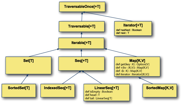
The collections hierarchy starts with the trait TraversableOnce. This trait represents a collection that can be traversed at least once. This trait abstracts between Traversable and Iterator. An Iterator is a stream of incoming items where advancing to the next item consumes the current item. A Traversable represents a collection that defines a mechanism to traverse the entire collection but can be traversed repeatedly. The Iterable trait is similar to Traversable but allows the repeated creation of an Iterator. The hierarchy branches out into sequences, maps (also known as dictionaries), and sets.

The Gen* Traits

In reality, the collection hierarchy has a duplicate generic variant. Every trait in the hierarchy has a Gen* trait that it inherits from, such as GenTraversableOnce, GenIterator, and GenSeq. The generic variants of collections offer no guarantees on serial or parallel execution, while the traits discussed here enforce sequential execution. The principles behind each collection are the same, but traversal ordering isn’t guaranteed for parallel collections. We discuss parallel collections in detail in section 8.4.2.

Let’s look at when to use each of the collection types.

8.1.2. Traversable

The Traversable trait is defined in terms of the foreach method. This method is an internal iterator—that is, the foreach method takes a function that operates on a single element of the collection and applies it to every element of the collection. Traversable collections don’t provide any way to stop traversing inside the foreach. To make certain operations efficient, the library uses preinitialized exceptions to break out of the iteration early and prevent wasted cycles. This technique is somewhat efficient on the JVM, but some simple algorithms will suffer greatly. The index operation, for example, has complexity O(n) for Traversable.

When using Traversables, it’s best to utilize operations that traverse the entire collection, such as filter, map, and flatMap. Traversables aren’t often seen in day-to-day development, but when they are, it’s common to convert them into another sort of collection for processing. For example, we’ll define a Traversable that opens a file and reads its lines for every traversal.

class FileLineTraversable(file: File) extends Traversable[String] {
  override def foreach[U](f: String => U) : Unit = {
    val input = new BufferedReader(new FileReader(file))
    try {
      var line = input.readLine
      while(line != null) {
        f(line)
        line = input.readLine
      }
    } finally {
      input.close()
    }
  }
  override def toString =
    "{Lines of " + file.getAbsolutePath + "}"
}

The FileLineTraversable class takes a file in its constructor and extends the Traversable trait for Strings. The foreach method is overridden to open the file and read lines from the file. The lines are passed into the function f. The method uses a try-finally block to ensure the file is closed after iteration. This implementation means that every time the collection is traversed, the file is opened and all of its contents are enumerated. Finally, the toString method is overridden so that when it’s called within the REPL, the entire file’s contents aren’t enumerated. Let’s use this class.

scala> val x = new FileLineTraversable(new java.io.File("test.txt"))
x: FileLineTraversable = {Lines of
/home/.../chapter8/collections-examples/test.txt}

scala> for { line <- x
     |   word <- line.split("\s+")
     | } yield word
res0: Traversable[java.lang.String] =
  List(Line, 1, Line, 2, Line, 3,
       Line, 4, Line, 5, ")

The first line constructs a FileLineTraversable against the test.txt file. This sample file contains lines that look like the following Line 1. The second line iterates over all the lines in the file and splits this line into words before constructing a new list with the words. The result is another Traversable of String that has all the individual words of the file.

The return type is Traversable even though the runtime type of the resulting list of words is a scala.List. The starting type in the for expression was a Traversable, so the resulting type of the expression will also be a Traversable without any outside intervention.

One concern with using the FileLineTraversable class is that the entire file would have to be traversed for any operation on the collection. Although we can’t create efficient random element access, the traversable can be terminated early if necessary. Let’s modify the definition of FileLineTraversable to include logging statements.

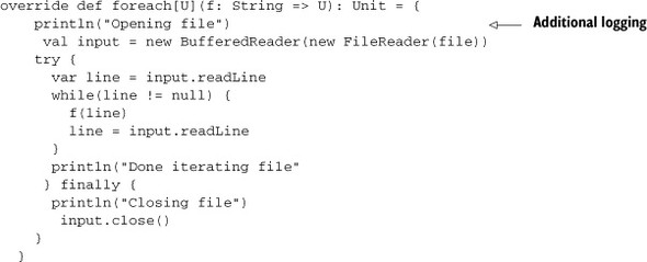
The foreach method has been modified with logging statements in three places: The first is when the file is opened, the second is when the file has reached its termination state, and the third is when the file is closed. Let’s see what happens with a previous example usage:

scala> val x = new FileLineTraversable(new java.io.File("test.txt"))
x: FileLineTraversable = {Lines of
  /home/.../scala-in-depth/chapter8/collections-examples/test.txt}

scala> for { line <- x
     |   word <- line.split("\s+")
     | } yield word
Opening file
Done iterating file
Closing file
res0: Traversable[java.lang.String] =
  List(Line, 1, Line, 2, Line, 3,
       Line, 4, Line, 5, ")

The FileLineTraversable is constructed the same as before. But now when trying to extract all the individual words, the logging statements are printed. The file is opened, the iteration is completed, and the file is closed. Now what happens if only the top two lines of the file need to be read?

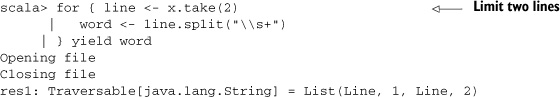
This time the take method is called against the FileLineTraversable. The take method is used to limit a collection to the first n elements, or in this case the first two elements. Now when extracting the lines of the file, the Opening file and Closing file logging statements print, but not the Done iterating file statement. This is because the Traversable class has an efficient means of terminating foreach early when necessary. We do this by throwing a scala.util.control.ControlThrowable. This preallocated exception can be efficiently thrown and caught on the JVM.

try { ... } catch {
 case ce : ControlThrowable => throw ce
 case t : Throwable => ...
}

The downside to this approach is that the take method will read three lines of the file before the exception is thrown to prevent continued iteration.

Traversable is one of the most abstract and powerful traits in the collections hierarchy. The foreach method is the easiest method to implement for any collection type, but it’s suboptimal for many algorithms. It doesn’t support random access efficiently and it requires one extra iteration when attempting to terminate traversal early. The next collection type, Iterable, solves the latter point by using an external iterator.

8.1.3. Iterable

The Iterable trait is defined in terms of the iterator method. This returns an external iterator that you can use to walk through the items in the collection. This class improves slightly on Traversable performance by allowing methods that need to parse a portion of the collection stop sooner than Traversable would allow.

External iterators are objects you can use to iterate the internals of another object. The Iterable trait’s iterator method returns an external iterator of type Iterator. The Iterator supports two methods, hasNext and next. The hasNext method returns true if there are more elements in the collection and returns false otherwise. The next method returns the next element in the collection or throws an exception if there are none left.

One of the downsides to having an external iterator is that collections such as the FileLineTraversable are hard to implement. The traversal of the collection is external to the collection itself, so the FileLineTraversable needs to know when all iterators are completed or no longer used before it can clean up memory/resources. In the worst case, the file may remain open for the entire life of an application. Because of this issue, subclasses of Iterable tend to be standard collections.

The major benefit of the Iterable interface is the ability to coiterate two collections efficiently. For example, let’s imagine that there are two lists. The first is a list of names and the second is a list of addresses. We can use the Iterable interface to iterate through both lists at the same time efficiently.

scala> val names = Iterable("Josh", "Jim")
names: Iterable[java.lang.String] = List(Josh, Jim)

scala> val address = Iterable("123 Anyroad, Anytown St 11111",
                                "125 Anyroad, Anytown St 11111")
address: Iterable[java.lang.String] =
  List(123 Anyroad, Anytown St 11111, 125 Anyroad, Anytown St 11111)

scala> val n = names.iterator
n: Iterator[java.lang.String] = non-empty iterator

scala> val a = address.iterator
a: Iterator[java.lang.String] = non-empty iterator

scala> while(n.hasNext && a.hasNext) {
     |   println(n.next + " lives at " + a.next)
     | }
Josh lives at 123 Anyroad, Anytown St 11111
Jim lives at 125 Anyroad, Anytown St 11111

The first line constructs an Iterable of name strings. The second line constructs an Iterable of address strings. The value n is created as an external iterator on the name strings. The value a is created as an external iterator on the address strings. The while loop iterates over both the a and n iterators simultaneously.

names.iterator zip address.iterator map { case (n, a) => n+" lives at
            "+a } foreach println

When joining information between two collections, requiring the Iterable trait can greatly improve the efficiency of the operation. But we still have an issue with using external iterators on mutable collections. The collection could change without the external iterator being aware of the change:

scala> val x = collection.mutable.ArrayBuffer(1,2,3)
x: scala.collection.mutable.ArrayBuffer[Int] = ArrayBuffer(1, 2, 3)

scala> val i = x.iterator
i: Iterator[Int] = non-empty iterator

The first line constructs a new ArrayBuffer collection (a mutable collection that extends from Iterable) with the elements 1, 2, and 3. Next, the value i is constructed as an iterator over the array. Now let’s remove all the elements from the mutable structure and see what happens to the i instance:

scala> x.remove(0,3)

scala> i.hasNext
res3: Boolean = true
scala> i.next
java.lang.IndexOutOfBoundsException: 0
...

The first line is a call to remove. This will remove all elements in the collection. The second line calls hasNext on the iterator. Because the iterator is external, it isn’t aware that the underlying collection has changed and returns true, implying there’s a next element. The next line calls the next method, which throws a java.lang.Index-OutOfBoundsException.

We should use the Iterable trait when explicit external iteration is required for a collection, but random access isn’t required.

8.1.4. Seq

The Seq trait is defined in terms of the length and apply method. It represents collections that have a sequential ordering. We can use the apply method to index into the collection by its ordering. The length method returns the size of the collection. The Seq trait offers no guarantees on performance of the indexing or length methods. We should use the Seq trait only to differentiate Sets and Maps from sequential collections—that is, if the order in which things are placed into a collections is important and duplicates should be allowed, then the Seq trait should be required.

A good example of when to use a Sequence is when working with sampled data, such as audio. Audio data is recorded at a sampling rate and the order in which it occurs is important in processing that data. Using the Seq trait allows the computation of sliding windows. Let’s instantiate some data and compute the sum of elements in sliding windows over the data.

scala> val x = Seq(2,1,30,-2,20,1,2,0)
x: Seq[Int] = List(2, 1, 30, -2, 20, 1, 2, 0)

scala> x.tails map (_.take(2)) filter (_.length > 1) map (_.sum) toList
res24: List[Int] = List(3, 31, 28, 18, 21, 3, 2)

The first line constructs an example input audio sequence. The second line computes the sum of sliding windows. The sliding windows are created using the tails method. The tails method returns an iterator over the tail of an existing collection. This means, each successive collection in the tails iterator has one less element. These collections can be converted into sliding windows using the take method, which ensures only N elements exist (in this case two). Next, we use the filter method to remove windows that are less than the desired size. Finally, the sum method is called on these windows and the resulting collection is converted to a list.

scala> Seq(2,1,30,-2,20,1,2,0).sliding(2).map(_.sum).toList
res0: List[Int] = List(3, 31, 28, 18, 21, 3, 2)

Sequence tends to be used frequently in abstract methods when the algorithms are usually targeted at one of its two subclasses: LinearSeq and IndexedSeq. We prefer these where applicable. Let’s look at LinearSeq first.

8.1.5. LinearSeq

The LinearSeq trait is used to denote that a collection can be split into a head and tail component. The trait is defined in terms of three “assumed to be efficient” abstract methods: isEmpty, head, and tail. The isEmpty method returns true if the collection is empty. The head method returns the first element of the collection if the collection isn’t empty. The tail method returns the entire collection minus the head. This type of collection is ideal for tail recursive algorithms that split collections by their head.

The canonical example of a LinearSeq is a Stack. A Stack is a collection that operates like a stack of toys. It’s easy to get the last toy placed on the stack, but it could be frustrating to continually remove toys to reach the bottom of the stack. A LinearSeq is similar in that it can be decomposed into the head (or top) element and the rest of the collection.

Let’s look at how we can use a LinearSeq as a stack in a tree traversal algorithm. First, let’s define a binary tree datatype.

sealed trait BinaryTree[+A]
case object NilTree extends BinaryTree[Nothing]
case class Branch[+A](value: A,
                      lhs: BinaryTree[A],
                      rhs: BinaryTree[A]) extends BinaryTree[A]
case class Leaf[+A](value: A) extends BinaryTree[A]

The trait BinaryTree is defined as covariant on its type parameter A. It has no methods and is sealed to prevent subclasses outside of the current compilation unit. The object NilTree represents a completely empty tree. It’s defined with the type parameter specified to Nothing, which allows it to be used in any BinaryTree. The Branch class is defined such that it has a value and a left-hand tree and right-hand tree. Finally, the Leaf type is defined as a BinaryTree that contains only a value. Let’s define an algorithm to traverse this BinaryTree.

def traverse[A, U](t: BinaryTree[A])(f: A => U): Unit = {
    @annotation.tailrec
    def traverseHelper(current: BinaryTree[A],
                      next: LinearSeq[BinaryTree[A]]): Unit =
      current match {
        case Branch(value, lhs, rhs) =>
          f(value)
          traverseHelper(lhs, rhs +: next)
        case Leaf(value) if !next.isEmpty =>
          f(value)
          traverseHelper(next.head, next.tail)
        case Leaf(value) => f(value)
        case NilTree if !next.isEmpty =>
          traverseHelper(next.head, next.tail)
        case NilTree => ()
      }
    traverseHelper(t, LinearSeq())
  }

The traverse method is defined to take a BinaryTree of content elements A and a function that operates on the contents and returns values of type U. The traverse method uses a nested helper method to implement the core of its functionality. The traverseHelper method is tail recursive and is used to iterate over all the elements in the tree. The traverseHelper method takes the current tree it’s iterating over and a nextLinearSeq, which contains the elements of the binary tree that it should look at later.

The traverseHelper method does a match against the current tree. If the current tree is a branch, it’ll send the value at the branch to the function f and then recursively call itself. When it does this recursive call, it passes the left-hand tree as the next node to look at and appends the right-hand tree to the front of the LinearSeq using the +: method. Appending the right-hand tree to the LinearSeq is a fast operation, usually O(1), due to the requirements of the LinearSeq trait.

If the traverseHelper method encounters a Leaf, the value is sent to the function f. But if the next stack isn’t empty, the stack is decomposed using the head and tail method. These methods are defined as efficient for the LinearSeq, usually O(1). The head is passed into the traverseHelper method as the current tree and the tail is passed as the next stack.

Finally, if the traverseHelper method encounters a NilTree it operates similarly to when it encounters a Leaf. Because a NilTree doesn’t contain data, only the recursive traverseHelper call is needed.

Now, let’s construct a BinaryTree and see what traversal looks like:

scala> Branch(1, Leaf(2), Branch(3, Leaf(4), NilTree))
res0: Branch[Int] = Branch(1,Leaf(2),Branch(3,Leaf(4),NilTree))

scala> BinaryTree.traverse(res0)(println)
1
2
3
4

First, a BinaryTree is created with two branches and two leaves. Next the Binary-Tree.traverse method is called against the tree with the method println for traversal. The resulting output is each value printed in the expected order: 1, 2, 3, 4.

This technique of manually creating a Stack on the Heap and deferring work onto it is a common practice when converting a general recursive algorithm into a tail recursive algorithm or an iterative algorithm. When using a functional style with tail recursion, the LinearSeq trait is the right collection to use. Let’s look at a similar collection, the IndexedSeq.

8.1.6. IndexedSeq

The IndexedSeq trait is similar to the Seq trait except that it implies that random access of collection elements is efficient—that is, accessing elements of a collection should be constant or near constant. This collection type is ideal for most general-purpose algorithms that don’t involve head-tail decomposition. Let’s look at some of the random access methods and their utility.

scala> val x = IndexedSeq(1, 2, 3)
x: IndexedSeq[Int] = Vector(1, 2, 3)

scala> x.updated(1, 5)
res0: IndexedSeq[Int] = Vector(1, 5, 3)

An IndexedSeq can be created using the factory method defined on the IndexedSeq object. By default, this will create an immutable Vector, described in section 8.2.1. IndexedSeq collections have an updated method that takes an index and a new value and returns a new collection with the value at the index updated. In the preceding example, the value at index 1 is replaced with the integer 5.

Indexing into an IndexedSeq is done with the apply method. In Scala, a call to an apply method can be abbreviated so that indexing looks like the following:

scala> x(2)
res1: Int = 3

The expression x(2) is shorthand for x.apply(2). The result of the expression is the value at index 2 of the collection x. In Scala, indexing into any type of collection, including arrays, is done with an apply method rather than specialized syntax.

Sometimes it’s more important to check whether or not a collection contains a particular item than it is to retain ordering. The Set collection does this.

8.1.7. Set

The Set trait denotes a collection where each element is unique, at least according to the == method. A Set is the ideal collection to use when testing for the existence of an element in a collection or to ensure there are no duplicates within a collection.

Scala supports three types of immutable and mutable sets: TreeSet, HashSet, and BitSet.

The TreeSet is implemented as a red black tree of elements. A red black tree is a data structure that attempts to remain balanced, preserving O(log2n) random access to elements. We find elements in the tree by checking the current node. If the current node is greater than the desired value, we check the left subbranch. If the current node is less than the desired value, then we check the right subbranch. If the elements are equal, then the appropriate node was found. To create a TreeSet, an implicit Ordering type class is required so that the less than and greater than comparisons can be performed.

The HashSet collection is also implemented as a tree of elements. The biggest difference is that the HashSet uses the hash of a value to determine which node in the tree to place an element. This means that elements that have the same hash value are located at the same tree node. If the hashing algorithm has a low chance of collision, HashSets generally outperform TreeSets for lookup speed.

The BitSet collection is implemented as a sequence of Long values. The BitSet collection can store only integer values. A BitSet stores an integer value by setting the bit corresponding to that value to true in the underlying Long value. BitSets are often used to efficiently track and store in memory a large set of flags.

One of the features of Sets in Scala is that they extend from the type (A) => Boolean—that is, a Set can be used as a filtering function. Let’s look at mechanisms to limit the values in one collection by another.

scala> (1 to 100) filter (2 to 4).toSet
res6: scala.collection.immutable.IndexedSeq[Int] = Vector(2, 3, 4)

The range of numbers from 1 to 100 is filtered by the Set of numbers from 2 to 4. Note that any collection can be converted into a set (with some cost) using the toSet method. Because a Set is also a filtering function, it can be passed directly to the filter function on the range. The result is that only the numbers 2 through 4 are found in the result of the filter call.

Although Scala’s Set collection provides efficient existence checking on collections, the Map collection performs a similar operation on key value pairs.

8.1.8. Map

The Map trait denotes a collection of key value pairs where only one value for a given key exists. Map provides an efficient lookup for values based on their keys:

scala> val errorcodes = Map(1 -> "O NOES", 2 -> "KTHXBAI", 3 -> "ZOMG")
errorcodes: scala.collection.immutable.Map[Int,java.lang.String] =
  Map(1 -> O NOES, 2 -> KTHXBAI, 3 -> ZOMG)

scala> errorcodes(1)
res0: java.lang.String = O NOES

The first statement constructs a map of error codes to error messages. The -> method is from an implicit defined in scala.Predef, which converts an expression of the form A -> B to a tuple (A,B). The second statement accesses the value at key 1 in the errorcodes map.

Scala’s Map has implementation types for HashMaps and TreeMaps. These implementations are similar to the HashSet and TreeSet implementations. The basic rule of thumb is that if the key values have an efficient hashing algorithm with low chance of collisions, then HashMap is preferred.

Scala’s Map provides two interesting use cases that aren’t directly apparent from the documentation. The first is that, similarly to Set, a Map can be used as a partial function from the key type to the value type. Let’s take a look.

scala> List(1,3) map errorcodes
res1: List[java.lang.String] = List(O NOES, ZOMG)

A list of values 1 and 3 is transformed using the errorcodes map. For each element in the list, a value is searched for in the errorcodes map. The result is a list of error messages corresponding to the previous list of error values.

Scala’s Map also provides the ability to specify a default value to return in the event a key doesn’t yet exist:

scala> val addresses =
     | Map("josh" -> "123 someplace dr").withDefaultValue(
     |   "245 TheCompany St")
addresses: collection.immutable.Map[String,String] =
  Map(josh -> 123 someplace dr)

scala> addresses("josh")
res0: java.lang.String = 123 someplace dr

scala> addresses("john")
res1: java.lang.String = 245 TheCompany St

The addresses map is constructed as the configuration of what mailing address to use for a username. The Map is given a default value corresponding to a local company address where most users are assumed to be located. When looking up the address for user josh, a specific address is found. When looking up the address for the user john, the default is returned.

In idiomatic Scala, we usually use the generic Map type directly. This may be due to the underlying implementation being efficient, or from the convenience of three-letter collection names. Regardless of the original reason, the generic Map type is perfect for general purpose development.

Now that the basic collection types have been outlined, we’ll look at a few specific immutable implementations.

8.2. Immutable collections

Immutable collections are the default in Scala and have many benefits over mutable collections in general purpose programming. In particular, immutable collections can be shared across threads without the need for locking.

Scala’s immutable collections aim to provide both efficient and safe implementations. Many of these collections use advanced techniques to ‘share’ memory across differing versions of the collection. Let’s look at the three most commonly used immutable collections: Vector,List, and Stream.

8.2.1. Vector

Vectors are the general-purpose utility collection of Scala. Vectors have a log₃₂(N) random element access, which is effectively a small constant on the JVM using 32-bit integer indexes. They’re also completely immutable and have reasonable sharing characteristics. In the absence of hard performance constraints, you should make Vectors the default collection. Let’s look at its internal structure to see what makes it an ideal collection.

Vectors are composed as a trie on the index position of elements. A trie is a tree where every child in a given path down the tree shares some kind of common key as shown in figure 8.2:

Figure 8.2. Example index trie with a branching factor of two

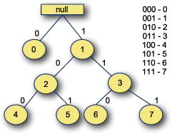
This is an example trie storing index values from 0 to 7. The root node of the trie is empty. Each node of the tree contains two values and a left and right branch. Each branch is labeled 0 or 1. The path to any index in the trie can be determined from the binary representation of the number. For example, the number 0 (000) is the 0th index element in the 0 branch from root, while the number 5 (101 in binary) is down the 1 branch from root, the 0 branch of the next node and the 1 branch of the final node. This gives us a well known path down the trie for any index given the binary number.

The binary trie can also be efficient. The cost of indexing any random element in the binary index trie is log₂(n), but this can be reduced by using a higher branching factor. If the branching factor was increased to 32, the access time for any element would be log₃₂(n), which for 32-bit indices is about 7 and for 64-bit indices is about 13. For smaller collections, due to the ordering of the trie, the access time is less. The random access time of elements scales with the size of the trie.

The other property of the trie is the level of sharing that can happen. If nodes are considered immutable, then changing values at a given index can reuse portions of the trie. Let’s take a look at this in figure 8.3.

Figure 8.3. Update to trie with sharing

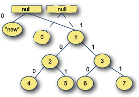
Here’s an updated trie where the value at index 0 is replaced with the value new. To create the new trie, two new nodes were created and the rest were reused as is. Immutable collections can benefit a great deal from sharing structure on every change. This can help reduce the overhead of changing the collections. In the worst case, the cost of changing a single element in the trie is log₂(n) for a branching factor of 2. This can be reduced by increasing the branching factor.

Scala’s Vector collection is similar to an indexed trie with a branch factor of 32. The key difference is that a Vector represents the branches of a trie as an array. This turns the entire structure into an array of arrays. Figure 8.4 shows what Scala’s Vector with branching factor of 2 would look like.

Figure 8.4. Vector’s array structure with branching factor of 2

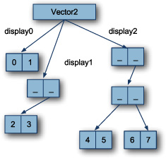
The binary branched Vector has three primary arrays: display0, display1, and display2. These arrays represent the depth of the original trie. Each display element is a successively deeper nested array: display0 is an array of elements, display1 is an array of an array of elements, and display2 is an array of an array of an array of elements. Finding an element in the collection involves determining the depth of the tree and indexing into the appropriate display array the same way that the binary trie was indexed. To find the number 4, the display depth is 2, so the display2 array is chosen. The number 4 is 100 in binary, so the outer array is indexed by 1, the middle array indexed by 0 and the number 4 is located at index 0 of the resulting array.

Because Scala’s Vector is branched 32 ways, it provides several benefits. As well as scaling lookup times and modification times with the size of the collection, it also provides decent cache coherency because elements that are near each other in the collection are likely to be in the same array in memory. Essential, like C++’s vector, Scala’s Vector should be the preferred collection for general-purpose computational needs. Its efficiency combined with the thread-safety gained from immutability make it the most powerful sequence in the library.

In some situations, Vector isn’t the most suited collection. When frequently performing head/tail decomposition, it’s better to use an immutable descendant of Scala’s LinearSeq trait: scala.collection.immutable.List

8.2.2. List

Scala’s immutable List collection is a singly linked list. This can have decent performance if you’re always appending or removing from the front of the list, but it can suffer with more advanced usage patterns. Most users coming from Java or Haskell tend to use List as a go-to default from habit. Although List has excellent performance in its intended use case, it’s less general than the Vector class and should be reserved for algorithms where it’s more efficient.

Let’s look at List’s general structure in figure 8.5.

Figure 8.5. Internal structure of a list

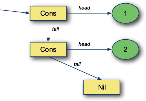
List is comprised of two classes: An empty list called Nil and a cons cell, sometimes referred to as a linked node. The cons cell holds a reference to a value and a reference to the rest of the list. Creating a list is as simple as creating cons cells for all the elements in the list. In Scala, the cons cell is called :: and the empty list is called Nil. A list can be constructed by appending elements to the empty list Nil.

scala> val x = 1 :: 2 :: 3 :: Nil
x: List[Int] = List(1, 2, 3)

This line appends 3 to the empty list and then appends 2 to that list and finally appends 1 to that list. The final effect is a linked list of 1, then 2, then 3. This uses a feature of Scala’s operator notation. If an operator ends with the : character, it’s considered right associative. The preceding line is equivalent to the following method calls:

scala> val x = Nil.::(3).::(2).::(1)
x: List[Int] = List(1, 2, 3)

In this version, it’s easier to see how the list is constructed. Scala’s treatment of the : character in operator notation is a general concept designed to handle cases like this where left associativity is not as expressive as right associativity.

The List collection extends from LinearSeq, as it supports O(1) head/tail decomposition and prepends.

Lists can support large amounts of sharing as long as you use prepends and head/tail decomposition. But if an item in the middle of the list needs to be modified, the front half of the list needs to be generated. This is what makes List less suited to general-purpose development than Vector.

List is also an eagerly evaluated collection. The head and tail components of a list are known when the list is constructed. Scala provides a different type of linked list where the values aren’t computed until needed. This collection is called a Stream.

8.2.3. Stream

Stream is a lazy persistent collection. A stream can lazily evaluate its members and persist them over time. A stream could represent an infinite sequence without overflowing memory constraints. Streams remember values that were computed during their lifetime, allowing efficient access to previous elements. This has the benefit of allowing backtracking but the downside of causing potential memory issues.

Scala’s Stream class is similar to Scala’s List class. A Stream is composed of cons cells and empty streams. The biggest difference between Stream and List is that Stream will lazily evaluate itself. Rather than storing elements, a stream stores function-objects that can be used to compute the head element and the rest of the Stream (tail). This allows Stream to store infinite sequences: a common tactic to join information with another collection. For example, this can be used to join indexes with elements in a sequence.

scala> List("a", "b", "c") zip (Stream from 1)
res5: List[(java.lang.String, Int)] = List((a,1), (b,2), (c,3))

The list of strings is zipped with an infinite stream of incrementing numbers starting from 1. The from method on Stream creates an infinitely incrementing stream starting at the passed in number. The zip method does pairwise join at each index element of two sequences. The result is that the elements of the original list are joined with their original indices. Even though the stream is infinite, the code compiles successfully because the stream is generated only for the indices required by the list.

Constructing a stream can be done similarly to list, except the cons (::) cell is constructed with the #:: method and an empty stream is referred to as Stream.empty. Let’s define a stream and see its execution behavior.

scala> val s = 1 #:: {
     |   println("HI")
     |   2
     | } #:: {
     |   println("BAI")
     |   3
     | } #:: Stream.empty
s: scala.collection.immutable.Stream[Int] = Stream(1, ?)

The stream s is created with three members. The first member is the number 1. The second is an anonymous function that prints HI and returns the value 2. The third is another anonymous function that prints BAI and returns the number 3. These three members are all prepended to an empty stream. The result is a stream of integers where the head is known to be the value 1. Notice that the strings HI and BAI aren’t printed. Let’s start accessing elements on the stream.

scala> s(0)
res39: Int = 1

scala> s(1)
HI
res40: Int = 2

scala> s(2)
BAI
res41: Int = 3

When accessing the first element in the stream, the head is returned without touching the rest of the stream. Nothing is printed to the console. But when the second index is accessed, the stream needs to compute the value. When computing the value, the string HI is printed to the console. Only the second value was computed. Next, when indexing into the third value, it must be computed and the BAI string is printed. Now, the stream has computed all of its elements.

scala> s
res43: scala.collection.immutable.Stream[Int] = Stream(1, 2, 3)

Now when printing the value of the stream to the console, it displays all three elements, because they’re persisted. The stream won’t recompute the values for indices it has already evaluated.

Lists in Haskell Versus Scala

One area of confusion when coming to Scala from Haskell is the List class. The Haskell language has lazy evaluation by default while Scala has eager evaluation by default. When looking for something from a lazily evaluated list, like Haskell’s list, use Scala’s Stream, not its List.

One excellent use of Streams is computing the next value of the stream using previous values. This is evident when calculating the Fibonacci sequence, which is a sequence where the next number is calculated using the sum of the previous two numbers.

scala> val fibs = {
     |   def f(a:Int,b:Int):Stream[Int] = a #:: f(b,a+b)
     |   f(0,1)
     | }
fibs: Stream[Int] = Stream(0, ?)

The fibs stream is defined using a helper function. The helper function f is defined to take two integers and construct the next portion of the Fibonacci sequence from them. The #:: method is used to prepend the first input number to the stream and recursively call the helper function f. The recursive call puts the second number in place of the first and adds the two numbers together to send in as the second number. Effectively, the function f is keeping track of the next two elements in the sequence and outputs one every time it’s called, delaying the rest of the calculation. The entire fibs sequence is created by seeding the helper function f with the numbers 0 and 1. Let’s take a look at the fib sequence:

scala> fibs drop 3 take 5 toList
res0: List[Int] = List(2, 3, 5, 8, 13)

scala> fibs
res1: Stream[Int] = Stream(0, 1, 1, 2, 3, 5, 8, 13, ?)

This method call drops the first three values of the sequence and takes five values from it and converts them to a list. The resulting portion of the Fibonacci sequence is displayed to the screen. Next, the fibs sequence is printed to the console. Notice that now the fibs sequence prints out the first eight elements. This is because those eight elements of Stream were evaluated. This is the persistence aspect of the Stream working.

Streams don’t work well when the eventual size of the stream won’t fit into memory. In these instances, it’s better to use a TraversableView to avoid performing work until necessary while allowing memory to be reclaimed. See section 8.1.1 for an example. If you need arbitrary high indices into a Fibonacci sequence, the collection could be defined as follows:

scala> val fibs2 = new Traversable[Int] {
     |   def foreach[U](f: Int => U): Unit = {
     |     def next(a: Int, b: Int): Unit = {
     |       f(a)
     |       next(b, a+b)
     |     }
     |     next(0,1)
     |   }
     | } view
fibs2: TraversableView[Int,Traversable[Int]] = TraversableView(...)

The fibs2 collection is defined as a Traversable of integers. The foreach method is defined in terms of a helper method next. The next method is almost the same as the helper method for the fibs stream except that instead of constructing a Stream, it loops infinitely, passing Fibonacci sequence values to the traversal function f. This Traversable is immediately turned into a TraversableView with the view method to prevent the foreach method from being called immediately. A view is a collection that lazily evaluates operations. Views are discussed in detail in section 8.4.1. Now, let’s use this version of a lazily evaluated collection.

scala> fibs2 drop 3 take 5 toList
res52: List[Int] = List(2, 3, 5, 8, 13)

scala> fibs2
res53: TraversableView[Int,Traversable[Int]] = TraversableView(...)

The same drop 3 take 5 toList methods are operated on the fibs2 collection. Similarly to Stream, the Fibonacci sequence is calculated on the fly and values are inserted into the resulting list. But when reinspecting the fibs2 sequence after operating on it, none of the calculated indices are remembered on the TraversableView. This means indexing into the TraversableView repeatedly could be expensive. It’s best to save the TraversableView for scenarios where a Stream would not fit in memory.

Stream provides an elegant way to lazily evaluate elements of a collection. This can amortize the cost of calculating an expensive sequence or allow infinite streams to be used. They’re simple and easy to use when needed.

Sometimes, mutating collections is necessary for performance reasons. Although mutability should and can be avoided in general development, it’s necessary in situations and can be beneficial. Let’s look at how to achieve mutability in Scala’s collection library.

8.3. Mutable collections

Mutable collections are collections that can conceptually change during their lifetime. The perfect example is an array. The individual elements of the array could be modified at any point during the array’s lifetime.

In Scala, mutability isn’t the default in the collections API. Using or creating mutable collections requires importing one or more interfaces from the scala.collections .mutable package and knowing which methods will mutate the existing collection vs. creating a new collection. For example, the map, flatMap, and filter methods defined on mutable collections will create new collections rather than mutate a collection in place.

The mutable collections library provides a few collections and abstractions that need to be investigated over and above the core abstractions:

• ArrayBuffer
• Mixin mutation event publishing
• Mixin serialization

Let’s start looking at ArrayBuffer.

8.3.1. ArrayBuffer

The ArrayBuffer collection is a mutable Array that may or may not be the same size as that of the collection. This allows elements to be added without requiring the entire array to be copied. Internally, an ArrayBuffer is an Array of elements, as well as the stored current size. When an element is added to an ArrayBuffer, this size is checked. If the underlying array isn’t full, then the element is directly added to the array. If the underlying array is full, then a larger array is constructed and all the elements are copied to the new array. The key is that the new array is constructed larger than required for the current addition.

Although the entire array is copied into the new array on some append operations, the amortized cost for append is a constant. Amortized cost is the cost calculated over a long time—that is, during the lifetime of an ArrayBuffer, the cost of appending averages out to be linear across all the operations, even though any given append operation could be O(1) or O(n). This property makes ArrayBuffer a likely candidate for most mutable sequence construction.

The ArrayBuffer collection is similar to Java’s java.util.ArrayList. The main difference between the two is that Java’s ArrayList attempts to amortize the cost of removing and appending to the front and back of the list whereas Scala’s ArrayBuffer is only optimized for adding and removing to the end of the sequence.

The ArrayBuffer collection is ideal for most situations where mutable sequences are required. In Scala, it’s the mutable equivalent of the Vector class. Let’s look at one of the abstractions in the mutable collections library, mixin mutation event publishing.

8.3.2. Mixin mutation event publishing

Scala’s mutable collection library provides three traits, ObservableMap, Observable-Buffer, and ObservableSet, that can be used to listen to mutation events on collections. Mixing one of these traits into the appropriate collection will cause all mutations to get fired as events to observers. These events are sent to observers, and the observers have a chance to prevent the mutation. Here’s an example:

scala>   object x extends ArrayBuffer[Int] with ObservableBuffer[Int] {
     |     subscribe(new Sub {
     |       override def notify(pub: Pub,
     |                           evt: Message[Int] with Undoable) = {
     |         Console.println("Event: " + evt + " from " + pub)
     |       }
     |     })
     |   }
defined module x

The object x is created as an ArrayBuffer that mixes in the ObservableBuffer. In the constructor, a subscriber is registered that prints events as they happen:

scala> x += 1
Event: Include(End,1) from ArrayBuffer(1)
res2: x.type = ArrayBuffer(1)

scala> x -= 1
Event: Remove(Index(0),1) from ArrayBuffer()
res3: x.type = ArrayBuffer()

Adding the element 1 to the collection causes the Include event to be fired. This event indicates that a new element is included in the underlying collection. Next the element 1 is removed from the collection. The result is a Remove event, indicating the index and value that was removed.

The full details of the event API for collection mutation is contained in the scala.collection.script package. The API is designed for advanced use cases such as data binding. Data binding is a practice where one object’s state is controlled from another object’s state. This is common in UI programming, where a list displayed onscreen could be tied directly to a Scala ArrayBufferwithObservableBuffer. That way, any changes to the underlying ArrayBuffer would update the display of the UI element.

Scala’s mutable collection library also allows mixins to be used to synchronize operations on collections.

8.3.3. Mixin synchronization

Scala defines the traits SynchronizedBuffer, SynchronizedMap, SynchronizedSet, SynchronizedStack, and SynchronizedPriorityQueue for modifying the behavior of mutable collections. A Synchronized* trait can be used on its corresponding collection to enforce atomicity of operations on that collection.

These traits effectively wrap methods on collections with a this.synchronized{} call. Although this is a neat trick to aid in thread safety, these traits are little used in practice. It’s better to use mutable collections in single threaded scenarios and promote immutable collections for cross thread data sharing.

Let’s look at an alternative solution to parallelizing and optimizing collection usage: Views and Parallel collections.

8.4. Changing evaluation with views and parallel collections

The base collection in the collection hierarchy defaults to strict and sequential evaluation. Strict evaluation is when operations are performed immediately when they’re defined. This is in contrast to lazy evaluation where operations can be deferred. Sequential evaluation is when operations are performed sequentially without parallelism against a collection. As shown in figure 8.6, this is in contrast to parallel evaluation where evaluation could happen on multiple threads across portions of the collection.

Figure 8.6. Changing evaluation semantics

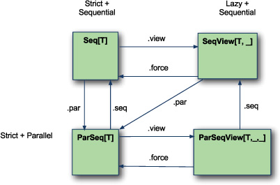
The collections library provides two standard mechanisms to migrate from the default evaluation semantics into either parallel or lazy evaluation. These take the form of the view and par methods. The view method can take any collection and efficiently create a new collection that will have lazy evaluation. The force method is the inverse of the view method. It’s used to create a new collection that has strict evaluation of its operations. Views will be covered in detail in section 8.4.1.

In a similar fashion, the par method is used to create a collection that uses parallel execution. The inverse of the par method is the seq method, which converts the current collection into one that supports sequential evaluation.

One important thing to note in the diagram is what happens when calling the par method on a View. As of Scala 2.9.0.1, this method call converts a sequential lazy collection into a parallel strict collection rather than a parallel lazy collection. This is due to how the encoding of types work. Let’s investigate this mechanism some more.

8.4.1. Views

The collections in the collections library default to strict evaluation—that is, when using the map method on a collection, a new collection is immediately created before continuing with any other function call. Collections views are lazily evaluated. Method calls on a view will only be performed when they absolutely have to. Let’s look at a simple example using List.

scala> List(1,2,3,4) map { i => println(i); i+1 }
1
2
3
4
res1: List[Int] = List(2, 3, 4, 5)

This line constructs a list and iterates over each of its elements. During this iteration, the value is printed and the value is modified by one. The result is that each element gets printed to the string and the resulting list is created. Let’s do the same thing, except this time we’ll change from using a List to a ListView.

scala> List(1,2,3,4).view map { i => println(i); i+1 }
res2: scala.collection.SeqView[Int,Seq[_]] = SeqViewM(...)

This expression is the same as the previous one, except the view method is called on List. The view method returns a view or window looking at the current collection that delays all functions as long as possible. The map function call against the view is not performed. Let’s modify the result so that the values are printed.

scala> res2.toList
1
2
3
4
res3: List[Int] = List(2, 3, 4, 5)

The toList method is called against the view from the previous example. Because the view must construct a new collection, the map function that was deferred before is executed and the value of each item of the original list is printed. Finally, the value of the new list, with each element incremented by one, is returned.

Views pair well with Traversable collections. Let’s reexamine the FileLineTraversable class from before. This class opens a file and iterates over the lines for every traversal. This can be combined with a view to create a collection that will load and parse a file when it’s iterated.

Let’s imagine that a system has a simple property configuration file format. Every line of a config file is a key-value pair separated by the = character. Any = character is considered a valid identifier. Also, any line that doesn’t have an = character is assumed to be a comment. Let’s define the parsing mechanism.

def parsedConfigFile(file: java.io.File) = {
    val P = new scala.util.matching.Regex("([^=]+)=(.+)")
    for {
      P(key,value) <- (new FileLineTraversable(file)).view
    } yield key -> value
  }

The parsedConfigFile takes in the config file to parse. The value P is instantiated as a regular expression. The expression matches lines that have a single = sign with content on both sides. Finally, a for expression is used to parse the file. A FileLineTraversable is constructed and the view method is called on this traversable, delaying any real execution. The regular expression P is used to extract key-value pairs and return them. Let’s try it out in the REPL.

scala> val config = parsedConfigFile(new java.io.File("config.txt"))
config: TraversableView[(String, String),Traversable[_]] =
  TraversableViewFM(...)

The parsedConfigFile method is called with a sample config file. The config contains two attribute value pairs that are numbered. Notice that the file isn’t opened and traversed. The return type is a TraversableView of (String,String) values. Now, when the configuration file should be read, the force method can be used to force evaluation of the view.

scala> config force
Opening file
Done iterating file
Closing file
res13: Traversable[(String, String)] =
  List((attribute1,value1), (attribute2,value2))

The force method is called on the config TraversableView. This causes strict evaluation of the deferred operations. The file is opened and iterated, pulling out all the parsable lines; these values are returned into the result.

Using views with Traversables is a handy way to construct portions of a program and delay their execution until necessary. For example, in an old Enterprise JavaBeans application, I constructed a parsable TraversableView that would execute an RMI call into the ApplicationServer for the current list of “active” data and perform operations on this list. Although there were several operations to whittle down and transform the data after it was returned from the ApplicationServer, these could be abstracted behind the TraversableView, similarly to how the config file example exposed a TraversableView of key value pairs rather than a TraversableView of the raw file.

Let’s look at another way to change the execution behavior of collections: parallelization.

8.4.2. Parallel collections

Parallel collections are collections that attempt to run their operations in parallel.

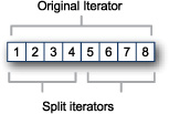
Parallel collections are implemented in terms of Splitable iterators. A Splitable iterator is an iterator that can be efficiently split into multiple iterators where each iterator owns a portion of the original iterator.

Figure 8.7 shows a Splitable iterator that originally points to a collection of the numbers 1 through 8. In the example, the Splitable iterator is split into two iterators. The first covers the numbers 1 through 4 and the second covers the numbers 5 through 8. These split iterators can be fed to different threads for processing.

Figure 8.7. Splitting parallel collection iterators

The Parallel collection operations are implemented as tasks on Splitable iterators. Each task could be run using a parallel executor, by default a ForkJoinPool, initialized with a number of worker threads equal to the number of processors available on the current machine. Tasks themselves can be split, and each task defines a threshold it can use to determine whether it should be split further.

Let’s look at figure 8.8 to see what might happen in parallel when calculating the sum of elements in a parallel collection.

Figure 8.8. Parallel task breakdown of sum method

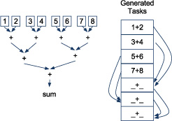
The sum method on the collection of one to eight is split into seven tasks. Each task computes the sum of the numbers below it. If a task contains more numbers than the threshold, assumed to be two in this example, the collection is split and more sum tasks are thrown on the queue.

These tasks are farmed out to a ForkJoinPool and executed in parallel. A ForkJoin-Pool is like a thread pool, but with better performance for tasks that fork (split) first and join (combine) later.

When using parallel collections, there are two things to worry about:

• The efficiency of converting from a sequential to a parallel collection
• The parallelizability of a task

The collections library does its best to reduce the cost of the first. The library defines a ParArray collection that can take Arrays, and Array-based collections, and convert them into their parallel variant. The library also defines a ParVector collection that can efficiently, in 0(1) time, convert from a Vector to a ParVector. In addition to these, the library has a mechanism to parallelize Set, Map, and the Range collections. The collections that aren’t converted efficiently are those that subclass from LinearSeq. Let’s take a look.

scala> List(1,2,3).par
res18: collection.parallel.immutable.ParSeq[Int] = ParVector(1, 2, 3)

In this example, a List of three numbers is converted to a parallel collection using the par method. The result is a ParVector. The runtime complexity of this operation is O(N) because the library has to construct a Vector from the List. If this overhead, combined with the overhead of parallelizing, is less than the runtime of an algorithm, it can still make sense to parallelize LinearSeq. But in most cases, it’s best to avoid LinearSeq and its descendants when using parallel collections.

The second thing to worry about with parallel collections is the parallelizability of a task. This is the amount of parallelism that can be expected from a given task. For example, the map method on collections can have a huge amount of parallelism. The map operation takes each element of a collection and transforms it into something else, returning a new collection. This is ideal for parallel collections.

scala> ParVector(1,2,3,4) map (_.toString)
res22: collection.parallel.immutable.ParVector[java.lang.String] =
  ParVector(1, 2, 3, 4)

The preceding constructs a parallel vector of integers and converts all the elements to their string representation.

One method that doesn’t have any parallelism is the foldLeft method. The fold-Left method on collections takes an initial value and a binary operation and performs the operation over the elements in a left-associative fashion. For example, given a collection of the values 1, 2, 3, and 4 and an initial value of 0, the binary operation + would be applied as follows: (((0 + 1) + 2) + 3)+ 4). The association requires that the operations be performed in sequence. If this were used on a parallel collection to compute the sum of elements in the collection, it would not execute in parallel. Let’s take a look:

scala> (1 to 1000).par.foldLeft(0)(_+_)
res25: Int = 500500

A parallel range is constructed with the values 1 through 1,000. The foldLeft method is called with an initial value of 0 and an operation of +. The result is the correct sum, but there’s no indication of whether this was parallelized. Let’s use a cheap trick to figure out if the foldLeft is parallelized.

scala> (1 to 1000).par.foldLeft(Set[String]()) {
     | (set,value) =>
     |    set + Thread.currentThread.toString()
     | }
res30: scala.collection.immutable.Set[String] =
  Set(Thread[Thread-26,5,main])

This time the foldLeft method is called with an empty Set of strings. The binary operation appends the current executing thread to the set. But if the same trick is used with the map operation, more than one thread will be displayed on a multicore machine:

scala> (1 to 1000).par map { ignore =>
     |   Thread.currentThread.toString
     | } toSet
res34: collection.parallel.immutable.ParSet[java.lang.String] = ParSet(
   Thread[ForkJoinPool-1-worker-0,5,main],
   Thread[ForkJoinPool-1-worker-1,5,main])

The parallel range from 1 to 1,000 is created and the map operation is called. The map operation converts each element to the current thread it’s running in, and the resulting list of threads is converted to a Set, effectively removing duplicates. The resulting list on my dual-core machine has two threads. Notice that unlike the previous example, the threads are from the default ForkJoinPool.

So, using parallel collections for parallelism requires using the parallelizable operations. The API documentation does a good job marking which operations are parallelizable, so it’s best to take a thorough read through the scaladoc in the scala.collection.parallel package.

With all these different collection types, it can be difficult to write generic methods that need to work against many collection types. We’ll discuss some mechanisms to do this.

8.5. Writing methods to use with all collection types

The new collections library goes to great lengths to ensure that generic methods, like map, filter, and flatMap will return the most specific type possible. If you start with a List, you should expect to retain a List for the duration of computations unless you perform some sort of transformation. You can do this property through a few type system tricks. Let’s look at implementing a generic sort algorithm against collections.

A naive approach would be the following:

object NaiveQuickSort {
  def sort[T](a: Iterable[T])(implicit n: Ordering[T]): Iterable[T] =
    if (a.size < 2) a
    else {
      import n._
      val pivot = a.head
      sort(a.filter(_ < pivot)) ++
      a.filter(_ == pivot) ++
      sort(a.filter(_ > pivot))
  }
}

The NaiveQuickSort object is defined with a single method sort. The sort method implements a quick sort. It takes in an Iterable of elements of type T. The implicit parameter list accepts the type class Ordering for the type T. This is what’s used to determine if one of the elements of the Iterable is larger, smaller, or equal to another. Finally, the function returns an Iterable. The implementation pulls a pivot element and splits the collection into three sets: elements less than the pivot, elements greater than the pivot, and elements equal to the pivot. These sets are then sorted and combined to create the final sorted list.

This algorithm works for most collections but has one obvious flaw:

scala> NaiveQuickSort.sort(List(2,1,3))
res12: Iterable[Int] = List(1, 2, 3)

The NaiveQuickSort.sort method is called with an unsorted List. The result is a sorted collection, but the type is Iterable, not List. The method does work, but the loss of the List type is undesirable. Let’s see if the sort can be modified to retain the original type of the collection, if possible.

object QuickSortBetterTypes {
  def sort[T, Coll](a: Coll)(implicit ev0: Coll <:< SeqLike[T, Coll],
                            cbf: CanBuildFrom[Coll, T, Coll],
                            n: Ordering[T]): Coll = {
    if (a.length < 2)
      a
    else {
      import n._
      val pivot = a.head
      val (lower : Coll, tmp : Coll) = a.partition(_ < pivot)
      val (upper : Coll, same : Coll) = tmp.partition(_ > pivot)
      val b = cbf()
      b.sizeHint(a.length)
      b ++= sort[T,Coll](lower)
      b ++= same
      b ++= sort[T,Coll](upper)
      b.result
    }
  }
}

The QuickSortBetterTypes object is created with a single method, sort. The guts of the algorithm are the same as before, except a generic builder is used to construct the sorted list. The biggest change is in the signature of the sort method, so let’s deconstruct it.

T is the type parameter representing elements of the collection. T is required to have an Ordering in this method (the implicit n : Ordering[T] parameter in the second parameter list). The ordering members are imported on the first line of the method. This allows the < and > operations to be “pimped” onto the type T for convenience. The second type parameters is Coll. This is the concrete Collection type. Notice that no type bounds are defined. It’s a common habit for folks new to Scala to define generic collection parameters as follows: Col[T] <: Seq[T]. Don’t do this, as this type doesn’t quite mean what you want. Instead of allowing any subtype of a sequence, it allows only subtypes of a sequence that also have type parameters (which is most collections). You can run into issues if your collection has no type parameters or more than one type parameter. For example:

object Foo extends Seq[Int] {...}
trait DatabaseResultSetWalker[T, DbType] extends Seq[T] {...}

Both of these will fail type checking when trying to pass them into a method taking Col[T] <: Seq[T]. For the object Foo, this is because it has no type parameters, but the constraint Col[T] <: Seq[T] requires a single type parameter. The DatabaseResultSetWalker trait can’t match Col[T] <: Seq[T] because it has two type parameters, where the requirement is for only one. Although there are workarounds, that requirement can be surprising to users of the function. The workaround is to defer the type-checking algorithm using the implicit system (see section 7.2.3).

To get the compiler to infer the type parameter on the lower bound, we have to defer the type inferencer long enough for it to figure out all the types. To do that, we don’t enforce the type constraint until we do the implicit lookup using the <:< class. The first implicit parameter ev0 : Coll <:< SeqLike[T, Coll] is used to ensure that the type Coll is a valid collection type with elements of T. This signature uses the SeqLike class. Although most consider the SeqLike classes to be an implementation detail, they’re important when implementing any sort of generic method against collections. SeqLike captures the original fully typed collection in its second type parameter. This allows the type system to carry the most specific type through a generic method so that it can be used in the return value.

Deferring Type Inference of Parent-Class Type Parameters

The need to defer the type inference for a type parameter Foo <: Seq[T] is necessary for supporting the Scala 2.8.x series. As of the Scala 2.9.x, the type inference algorithm was improved such that the implicit <:< parameter is no longer necessary.

The next type parameter in the sort method is the cbf : CanBuildFrom[Coll, T, Coll]. The CanBuildFrom trait, when looked up implicitly, determines how to build new collections of a given type. The first type parameter represents the original collection type. The second type parameter represents the type of elements desired in the built collection—that is, the type of elements in the collection the method is going to return. The final type parameter of CanBuildFrom is the full type of the new collection. This is the same type as the input collection in the case of sort, because the sort algorithm should return the same type of collection that came in.

The CanBuildFrom class is used to construct the builder b. This builder is given a sizeHint for the final collection and is used to construct the final sorted collection rather than calling the ++ method directly. Let’s look at the final result.

scala> QuickSortBetterTypes.sort(
     |   Vector(56,1,1,8,9,10,4,5,6,7,8))
res0: scala.collection.immutable.Vector[Int] =
  Vector(1, 1, 4, 5, 6, 7, 8, 8, 9, 10, 56)

scala> QuickSortBetterTypes.sort(
     |   collection.mutable.ArrayBuffer(56,1,1,8,9,10,4,5,6,7,8))
res1: scala.collection.mutable.ArrayBuffer[Int] =
  ArrayBuffer(1, 1, 4, 5, 6, 7, 8, 8, 9, 10, 56)

The first line calls the new sort method against an unordered Vector of Ints. The resulting type is also a Vector of Ints. Next, the sort method is called against an ArrayBuffer of Ints. The result is again an ArrayBuffer of Ints. The new collection method now preserves the most specific type possible.

def foo[T, Coll <: LinearSeqLike[T, Coll]](t : Coll with
LinearSeqLike[T,Coll]) : Option[(T, Coll)]

This implementation of sort is generic but may be suboptimal for different types of collections. It would be ideal if the algorithm could be adapted such that it was optimized for each collection in the hierarchy. This is easy to do as a maintainer of the collections library, because the implementations can be placed directly on the classes. But when developing new algorithms outside the collections library, type classes can come to the rescue.

8.5.1. Optimizing algorithms for each collections type

You can use the type class paradigm to encode an algorithm against collections and refine that algorithm when speed improvements are possible. Let’s start by converting the generic sort algorithm from before into a type class paradigm. First we’ll define the type class for the sort algorithm.

trait Sortable[A] {
    def sort(a : A) : A
  }

The Sortable type class is defined against the type parameter A. The type parameter A is meant to be the full type of a collection. For example, sorting a list of integers would require a Sortable[List[Int]] object. The sort method takes a value of type A and returns a sorted version of type A. The generic sort method can now be modified to look as follows:

object Sorter {
  def sort[Col](col : Col)(implicit s : Sortable[Col]) = s.sort(col)
}

The Sorter object defines a single method sort. The generic sort method now takes in the Sortable type class and uses it to sort the input collection. Now the implicit resolution of default Sortable types needs to be defined.

trait GenericSortTrait {
  implicit def quicksort[T,Coll](
        implicit ev0: Coll <:< IterableLike[T, Coll],
        cbf: CanBuildFrom[Coll, T, Coll],
        n: Ordering[T]) =
    new Sortable[Coll] {
      def sort(a: Coll) : Coll =
        if (a.size < 2)
          a
        else {
          import n._
          val pivot = a.head
          val (lower: Coll, tmp: Coll) = a partition (_ < pivot)
          val (upper: Coll, same: Coll) = tmp partition (_ > pivot)
          val b = cbf()
          b.sizeHint(a.size)
          b ++= sort(lower)
          b ++= same
          b ++= sort(upper)
          b.result
        }
    }

The GenericSortTrait is defined to contain the implicit look up for the generic QuickSort algorithm. It has the single implicit method quicksort. The quicksort method defines the same type parameters and implicit parameters as the original sort method. Instead of sorting, it defines a new instance of the Sortable type trait.

The Sortable.sort method is defined the same as before. Now the GenericSort-Trait has to be placed onto the Sortable companion object so that it can be looked up in the default implicit resolution.

object Sortable extends GenericSortTrait

The Sortable companion object is defined to extend the GenericSortTrait. This places the implicit quicksort method in the implicit lookup path when looking for the Sortable[T] type trait. Let’s try it out.

scala> Sorter.sort(Vector(56,1,1,8,9,10,4,5,6,7,8))
res0: scala.collection.immutable.Vector[Int] =
  Vector(1, 1, 4, 5, 6, 7, 8, 8, 9, 10, 56)

The Sorter.sort method is called. The appropriate Sortable type trait is found for Vector and the collection is sorted using the quicksort algorithm. But if we try to call the sort method against something that doesn’t extend from IterableLike, it won’t work. Let’s try the sort method on Array.

scala> Sorter.sort(Array(2,1,3))
<console>:18: error: could not find implicit value for
  parameter s: Sorter.Sortable[Array[Int]]
       Sorter.sort(Array(2,1,3))

The Sorter.sort method is called with an unsorted array. The compiler complain that it can’t find a Sortable instance for Array[Int]. This is because Array does not extend from Iterable. Scala provides an implicit conversion that will wrap an Array and provide it with standard collection methods. Let’s provide an implementation of sort for Array. For simplicity, we’ll use a selection sort.

trait ArraySortTrait {
  implicit def arraySort[T](implicit mf: ClassManifest[T],
                            n: Ordering[T]): Sortable[Array[T]] =
    new Sortable[Array[T]] {
      def sort(a : Array[T]) : Array[T] = {
        import n._
        val b = a.clone
        var i = 0
        while (i < a.length) {
          var j = i
          while (j > 0 && b(j-1) > b(j)) {
            val tmp = b(j)
            b(j) = b(j-1)
            b(j-1) = tmp
            j -= 1
          }
          i += 1
        }
        b
      }
    }
}

The trait ArraySortTrait is defined with a single method arraySort. This method constructs a Sortable type trait using a ClassManifest and an Ordering. Using raw Arrays in Scala requires a ClassManifest so that the bytecode will use the appropriate method against the primitive arrays. The Sortable type trait is parameterized against Arrays. The algorithm loops through each index in the array and looks for the smallest element in the remainder of the array to swap into that position. The selection sort algorithm isn’t the most optimal, but it’s a common algorithm and easier to understand than what’s used classically in Java. This Sortable implementation needs to be added to the appropriate companion object for implicit resolution.

object Sortable extends ArraySortTrait with QuickSortTrait

The Sortable companion object is expanded to extend from both the ArraySortTrait, containing the Sortable type class for Array, and the QuickSort trait, containing the Sortable type class for iterable collections. Let’s use this implementation now.

scala> Sorter.sort(Array(2,1,3))
res0: Array[Int] = Array(1, 2, 3)

Now, when calling the sort method with Arrays, the call succeeds. You can use this technique to support any number of collections and to specialize behavior for collections using techniques shown in section 7.3.

Scala provides all the right tools to generically deal with collections. The complexity of doing so can be high, so it’s a judgment call when and how much abstraction is required for a particular method against collections.

8.6. Summary

The Scala collections library is one of the most compelling reasons to use Scala. From the power and versatility of the collection to the ability to preserve specific types on generic methods, Scala collections provide a clean and elegant solution to most problems. Using the collections API is a matter of understanding what the various type signatures mean and knowing how to flow between collection semantics and evaluation styles. Although the API is geared for immutability, there’s more than enough support for mutable collections and interfaces.

This chapter provides a great introduction to the key concepts behind the collections API, but knowing the methods defined on the collections and how to string them together is also important. Because the collections library is always improving, the best source for learning these methods is the scaladoc documentation for the current release.

The next chapter covers Scala actors, which are another important concept in the Scala ecosystem.