11

Integration Testing

The purpose of this chapter is to introduce the objectives of integration testing and the techniques used. Integration testing occurs when two or more modules, components, or subsystems are combined to form a new subsystem or a system. During the integration testing phase it is generally assumed that the components being integrated have been tested independently. Hence, the focus in this phase is on errors that may exist due to communication among components being integrated. Often, when many components are being integrated, one needs to determine their integration sequence. Three algorithms to determine an optimal or a near-optimal integration sequence are described and compared in this chapter.

11.1  Introduction

This chapter is concerned with issues that relate to integration testing. This type of testing refers to a testing activity wherein two or more components of a software system are tested together. A software component is sometimes also referred to as a class, a collection of classes, a module, a collection of methods, and so on. In integration testing a component might be as simple as a class in Java, or a file consisting of methods in C. Or, it could be as complex as a collection of many Java or C++ classes or several files each containing multiple methods in C.

 

Goal of integration testing: The goal of integration testing is to discover any problems that might arise when the components are integrated. Thus, for example, components C1 and C2 might have been tested and found to function correctly. However, this does not guarantee that when integrated, C1 and C2 will perform as expected. An error discovered during integration testing is often referred to as integration error. Hence the goal of integration testing is to discover any integration errors when two or more components are combined into a system or a subsystem. Of course, during integration testing one might discover an error in one of the components that had been tested previously. However, integration errors are those that would likely be revealed only when the components are integrated and tested together.

 

When does integration testing occur? Integration testing occurs at various levels. A developer might code a class C1 and test it. The same developer might then code class C2 that uses C1, and test both C1 and C2 as an integrated unit. This process may continue as the developer moves toward the goal of creating a reasonably complex component that consists of two or more classes. At a much higher level, a team of testers might integrate two or more complex components, or subsystems, perhaps developed by different teams within an organization. In yet another case, such a team of testers might integrate and test several components developed in-house with one or more components obtained from different sources.

 

Regardless of the level at which integration testing occurs, one faces a set of problems that ought to be solved prior to initiating the test. The following questions that arise during integration testing are considered in the remainder of this chapter.

 

1. Integration hierarchy: Should the components be integrated top-down, bottom-up, or using a mix of these two approaches?
2. Sequencing and stubbing: In what sequence should the components be integrated and what stubs are needed?
3. Test generation: What methods should be used to generate tests and to measure their adequacy?

In the remainder of this chapter, the terms class, component, and module are used synonymously unless differentiated explicitly.

11.2  Integration Errors

During integration testing, it is assumed that the components being integrated have been tested well, though independently. Thus, integration tests focus on the connections across the components being integrated. It is therefore useful to know what types of errors one might encounter during integration testing. Despite the fact that components being integrated have been tested, they might contain errors the impact of which is visible only when the components are integrated. Such errors are known as integration errors. Of course, one cannot deny the possibility that such errors may be found in unit testing. However, integration testing offers yet another opportunity to discover such errors.

 

Figure 11.1 shows the consequence of four types of integration errors. The figure offers a high level classification of the consequence of errors in components being integrated. Indeed, some of the errors that lead to the incorrect values shown in Figure 11.1 should have been found in unit testing. However, when the units are tested with stubs, incorrect values at the interfaces might go unchecked and revealed only during integration testing.

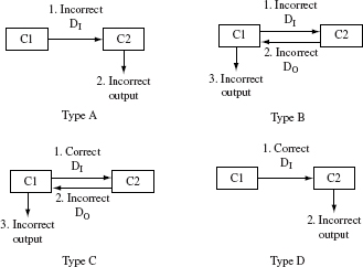
Figure 11.1 Types of integration errors. D_I is a set or a sequence of inputs passed from component C1 to component C2. D_O is a set or a sequence of outputs returned from component C2 to component C1.

Type A behavior in Figure 11.1 is a consequence of an error in component C1 and perhaps also in component C2. Type B behavior extends Type A by assuming that component C1 responds incorrectly and consequently results in an incorrect response from component C1. Type C behavior implies an error in component C2 and perhaps also in C1. Lastly, Type D behavior implies an error in C2.

Example 11.1   Consider the errors that may lead to the four types of behaviors exhibited in Figure 11.1. Events in the figure are numbered indicating the sequence in which they occur. Suppose that a call from C1 to a method in C2 sends incorrect parameter values (event 1). In turn, C2 computes incorrect results (event 2). This error in C1 leads to Type A behavior. Type B behavior results from a similar error but when C1 receives an incorrect result from C2 (event 2) it also generates an incorrect output (event 3). In either of these two cases, it is clear that C1 has an error but C2 might or might not.

Type C behavior could occur due to any one of several types of coding errors that lead to an incorrect output that in turn leads to an incorrect output from C1. Type D behavior is similar to Type C except that the incorrect output of C2 does not affect C1.

 

The categorization of different interface behaviors as in Figure 11.1 during integration testing is useful when assessing the adequacy of integration tests. Such adequacy assessment, using a powerful technique known as interface mutation, is discussed briefly in Chapter 8.

11.3  Dependence

Classes and collections of classes, better known as components, to be integrated are often related to each other leading to inter-class or inter-component dependencies. For example, class C1 might generate data and write it to a file. Class C2 might read the data written by C1 and perform further processing. In this example, C2 depends on data generated by C1 and hence we say that there exists data dependency between C1 and C2. In another case, C1 might make use of a function in C2 thus resulting in functional dependency. In yet another case, C1 might evaluate a condition that affects whether or not C2 is executed thus resulting in control dependence.

 

Dependence among classes and components has an impact on the sequence in which they are integrated and tested. In the remainder of this section we define different types of dependencies among classes in an object-oriented application such as those written in Java, C#, or C++. The type of dependence among classes is used in Section 11.6 in the algorithms for determining a component integration sequence. The dependences mentioned here are applicable to a collection of classes as well as a collection of components each of which might be a collection of one or more classes.

 

Figure 11.2 shows a graphical means of representing relationships among components. Such a graph is also known as Object Relation Diagram, or simply referred to as an ORD. We use the notation in Figure 11.2(a) or (b) when there is no need to specify the type of relationship and (c) when the specific relationship is of importance. Recall that a component could be as small as a class or as large as a subsystem. The algorithms presented in Section 11.6 are likely to be of practical use when the components to be integrated are fairly complex rather than simple classes. Nevertheless, these algorithms can be used regardless of the complexity of the components to be integrated.

 

While an ORD is a useful means to exhibit inter-component relations, it is certainly not the only means. Several details of component interactions are difficult or nearly almost impossible to describe in an ORD. In such cases, one uses textual means to describe the details of the interfaces. One such document, used by NASA when developing software systems for its spacecraft, is known as Interface Control Document, abbreviated as ICD. In the automobile industry, the AUTOSAR standard specified interfaces using Interface Files or the Software Specification (SWS) documents.

Figure 11.2 (a) Component C1 depends on component C2. (b) Components C1 and C2 depend on each other thus creating a cycle. (c) Component C1 depends on component C2 and the dependency type is T. Here T denotes some form of dependency described in Section 11.3.1. 

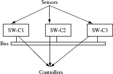
Example 11.2   Automobile engine control systems perform a number of time-dependent tasks. Often these tasks are performed by software components that are connected with each other over a network bus. As shown in Figure 11.3, a software component might receive data from one or more sensors and send control signals to an automobile component via one or more controllers.

 

ORDs can be used to express object relationships in an embedded system consisting of hardware and software.

In an environment like the one described above, each software component is treated as a black box. The actual code of the component might not be available though one assumes that the component itself has been well tested prior to integration testing. Thus, it might not be possible, or even feasible, to obtain a precise ORD for the components such as the one shown later in Figure 11.6. However, given the interface description, it should be possible to create a component dependence diagram that is similar to an ORD but that indicates dependence and not necessarily its type. Integration testing in such cases is based on precise interface requirements.

 

Obtaining precise relationships among objects might not always be possible, and especially so when the complete code of the system under test is unavailable.

For example, it might be required that SW-C1 obtains data from a sensor, processes it within 100 milliseconds, and sends a suitable message to SW-C2. In turn, SW-C2 consults a table, generates, and sends another data item to SW-C3. This component in turn computes a signal value from the data received and sends it to a controller. In this case, we know the dependencies among the various software components, sensors, and controllers. Hence a component dependence diagram can be drawn and used to decide a suitable integration sequence.

Figure 11.3 A partial chain consisting of software components in the engine control management of an automobile engine control management. Three software components (prefixed as SW-C) are shown. The components communicate via a bus. They also gather data from sensors and send signals to controllers.

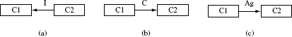
Figure 11.4 (a) Class C2 inherits from class C1. (b) Class C1 aggregates objects of class C2. (c) Class C1 uses data and or methods in class C2.

11.3.1  Class relationships: static

Classes in an object-oriented program are often related to each other. In its most generic form, such a relation is referred to as an association. During integration testing, it is sometimes useful to consider three types of relations: inheritance, aggregation, and association. The aggregation relationship is also known as composition.

 

The inheritance relation indicates that a class C2 inherits data and or methods from another class C1. As in Figure 11.4(a), the inheritance relationship is indicated by drawing an arrow from C2 to C1 and labeling it as “I” meaning that C2 inherits from C1. For example, in Java, class C2 can be made to inherit from class C1 by writing the class header as follows:

 

public class C2 extends C1{ // Extension of C1

. . . .

}

 

Figure 11.4(b) indicates that class C1 aggregates objects of class C2. Note that we label the arrow from C1 to C2 as “Ag.” For example, a class named Graph denoting a graph may aggregate objects of type Node. Further, Node might aggregate objects of type Edge. As another example, a class named Picture might aggregate several objects of type Point. The following code segment indicates aggregation of C2 objects:

 

public class C1 {

C2[ ] C2Objects = new C2[100]; // Aggregation of C2 objects.

C2 aC2Object = new C2; // C1 uses a C2 object.

. . . .

}

 

Figure 11.4(c) indicates that class C1 has an association with class C2 meaning thereby that C1 uses some data or method in C2. The association edge is labeled “As.” The following code segment indicates three possible ways in which C1 can associate itself with C2:

 

public class C1 {

. . .

int d = C2.getVal( ); // Use of method getVal( ) in C2.

float p = C2.x+1; // C1 accesses x in C2.

public void aMethod(C2 z); // C1 uses a field in C2.

. . . .

}

 

The first of the above three statements indicates method call association as class C1 uses a method in class C2. The second statement indicates field access association as class C1 uses variable x defined in C2. The last statement is an example of parameter association as class C1 uses a parameter of type C2 in method aMethod. It may be worth noting that aggregation is also a kind of association. However, in integration testing it is sometimes useful to distinguish among different types of associations as explained above.

It is also possible for a class to have more than one type of dependence on another class. Consider, for example, the following statements:

 

public class C1 {

public void method mC( ){ . . . }

. . .

}// End of C1

public class C2 extends C1 {

public C2( C1 c){c.mC( );}

. . .

}// End of C2

 

Clearly, in the above code segment, in an ORD, C2 has an edge to class C1 labeled I. In addition, due to the parameter c in the constructor, C2 also associates with C1. In such cases the edge from C2 to C1 can be labeled I/As.

11.3.2  Class relationships: dynamic

The relationships shown in an ORD can be derived at compile time. Hence, these are known as static relationships. However, when testing a collection of classes, it is important to know class dependencies that arise due to polymorphism or indirection. Such dependence of one class on the other is also known as dynamic dependence. The following example illustrates dynamic dependence.

Figure 11.5 (a) Static dependence ORD. (b) Dynamic dependence ORD derived from (a). 

Example 11.3   Figure 11.5(a) shows the relationships among seven classes labeled A through G. Note that classes C and D are subclasses of class B. Class A associates with class B and hence, due to polymorphism, it also associates with classes C, D, and G as shown in Figure 11.5(b). Further, class B aggregates objects of class F. Hence, transitively, class A also depends on class F.

The ORD in Figure 11.5(b) suggests that if, for example, class F is changed, then class B as well as class A ought to be tested. Similarly, when any of classes C, D, and G is modified, A needs to be retested.

11.3.3  Class firewalls

A firewall for class X is the set of all classes that may be affected if X is modified. Thus, any class that depends on X will be in the class firewall of X. Firewalls can be determined from the ORD. Let F_x denote the firewall for class X. All classes in F_x are targets for retesting when X is modified. Thus, firewalls are useful in determining what to test during regression as well as integration testing.

 

It is easy to determine a class firewall from an ORD using the following depends relation D:

 

D = {(X,Y)|when there is an edge in the ORD from class Y to class X}.

 

Let D⁺ denote the irreflexive transitive closure of D defined as follows:

 

D⁺ = {(X, Z)|(X, Y) and (Υ, Z) ∈ D}.

 

Using D we can define the firewall F_x for class X as follows:

 

F_X = {Z|(X, Z) ∈ D⁺}

Example 11.4   Let us determine the firewalls of all classes in Figure 11.5(a). Relations D and D⁺ can be computed by an examination of the ORD as follows:

 

An ORD can be used to determine the firewall of each class using a “depends” relation.

D = {(B, A), (E, B), (F, B), (B, C), (B, D), (D, C), (D, G)}.

D⁺ = D ∪ {(B, G), (E, C)(E, D), (E, G), (F, C)(F, D), (F, G)}.

 

Using D⁺ as above, the firewalls for each class in Figure 11.5(a) can be computed as follows:

11.3.4  Precise and imprecise relationships

An ORD can be derived from design diagrams during the early stages of software development. For example, class diagrams in UML could be a source of an ORD for an application. However, such an ORD is likely to be imprecise in the sense that it might show relationships that do not actually exist in the application code. Of course, this imprecision could be despite the fact that the application conforms to the design. While such an imprecise ORD is useful in generating integration test plans and for advance test planning, it might indicate stubs that are not needed. Hence, an ORD generated from a design is best useful for early planning, but not necessarily for the determination of the actual integration order, or regression test, or for code coverage analysis.

 

Once the application code is available, it is possible using static analysis of the code to refine the ORD constructed using the design. In some cases, one might like to construct a new ORD from the code. The ORD created from the code will likely exhibit a more accurate set of inter-class relationships than the ORD created using only the design. Of course, keep in mind that sometimes one reason why stubs are created is because the corresponding code is not available. In such a situation, one needs to rely on a mix of the design diagrams and whatever code is available.

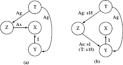
Figure 11.6 ORDs corresponding to Program P11.1. (a) Imprecise ORD. (b) Precise ORD.

Example 11.5   Consider a Java Program P11.1. It contains five classes. Class T is the top level class for testing the remaining classes. Class Y is a subclass of X. Class Z makes use of an object of type X in its constructor. Figure 11.6(a) shows an ORD assumed to be developed from the design diagram of this program. It shows the appropriate edges between the various classes.

Program P11.1

An examination of Program P11.1 reveals that T creates an object of type Z by passing an object of type Y. Further, an examination of the code of all classes reveals that Z will never actually use an object of type X. Thus, it is more appropriate to indicate an association relationship between Z and Y than to show a relationship between Z and X. This more precise relationship is shown in Figure 11.6(b).

The precise ORD in Figure 11.6(b) also shows exactly where the dependencies arise. For example, it shows that the dependence of T on Z is from the statement at line 18. Similarly, it also shows that the dependence of Z on Y is from the statement at line 12 in Z and the statement at line 18 in T.

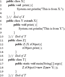
Precise ORDs are helpful in several situations. First, they help determine exactly which classes ought to be stubbed. Second, they help determine which portion of the class code ought to be covered when integrating two classes. And thirdly, during regression testing they help determine which classes ought to be retested when there is a change in one or more classes.

11.4  OO versus Non-OO Programs

The class relationships mentioned above are obviously for object-oriented (OO) programs written in languages such as Java and C++. In non-OO languages such as C, one can use other types of dependence graphs. For example, a call graph can be used to capture the dependence among various methods in a program. Note that a call graph can also be constructed for OO-programs. In fact a precise association relation between two objects indicates, among others, the calling relationships among methods across various objects.

 

For the purpose of integration testing, the call graph can be constructed so that only calls across different components to be integrated are captured while those within a component are ignored. Program dependence graphs introduced in Chapter 1 can be used to capture more precise dependence relationships such as data and control dependence.

Once the dependence among various components is captured, algorithms described in Section 11.6 can be used to help arrive at a test order. This order may simply be derived assuming an abstract dependence such as “component A depends on component B.” More detailed dependence types could also be used, such as “component A calls a method in component B.” While the abstract dependence is useful in deriving a test order, the more precise dependence is useful in deriving the tests and assessing their adequacy.

 

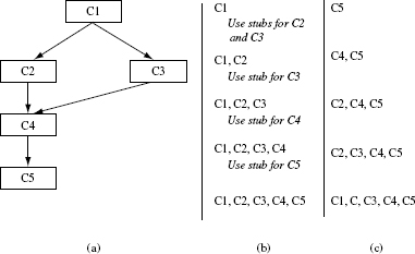
Figure 11.7 (a) A hypothetical set of classes and their relationships. (b) A sample top-down integration sequence. (c) A sample bottom-up integration sequence; drivers are needed for C5, C4, C2, and C3.

11.5  Integration Hierarchy

There are several strategies for integrating components prior to testing. Three strategies, namely, big-bang, top-down, and bottom-up, are explained next using the class hierarchy in Figure 11.7.

 

Big-bang integration: The big-bang strategy is to integrate all components in one step and test the entire system. Doing so does save time in writing stubs and drivers. When using this strategy for the system in Figure 11.7(a), all five classes shown will be integrated and tested together.

When using the big-bang strategy the identification of sources of failure, and correcting the errors, becomes increasingly more difficult with the complexity of the system. One may use this strategy when the number of components involved is small and each is relatively simple. Thus, big-bang integration might be useful when an individual programmer is testing self-designed and coded components of a large system.

 

It is important to note that big-bang integration testing is not the same as system testing. The goal in integration testing is to ensure that there are no integration errors, whereas in system testing one tests the entire system with several other objectives such as the correctness of the system level functionality, performance, and reliability.

Top-down integration: As the name implies, a strictly followed top-down integration strategy requires that components be integrated from the top moving down in the class hierarchy. Thus, for the hierarchy in Figure 11.7(a), one would begin testing class C1, then integrate it with C2 or C3, and test the combination {C1, C2} or {C1, C3} as the case may be. In the next step, the set of classes {C1, C2, C3} are integrated and tested. Finally, the complete set of five classes will be tested. As shown in Figure 11.7(b), top-down testing requires the use of stubs. Thus, when testing C1 alone, one needs stubs for C2 and C3 because C1 depends on C2 and C3. Similarly when testing the combination {C1, C2, C3}, one needs stubs for class C4.

 

In the above, we have described a strict interpretation of top-down integration. In practice, the test team might decide to integrate in one of many different ways. For example, if classes C1, C2, and C3 are all available and have been individually tested, then they can be integrated and tested together. In the next step, assuming that classes C4 and C5 are available, the entire set of classes can be integrated and tested. Thus, instead of using the steps described earlier, one may perform the integration in only two steps. Toward the end of this section we examine the factors that help a test team decide what to integrate and when.

Bottom-up integration: In strict bottom-up integration one moves up the component hierarchy to integrate and test components. As shown in Figure 11.7(c), class C5 is tested first. Next, C1 is integrated with C4 and the combination tested. The integration proceeds until all components have been integrated and tested. Bottom-up testing requires the creation of drivers. For example, when testing C5, one needs a driver to make “use of” or to “drive” the execution of code in C5 that is used by classes that depend on it. Thus, whereas top-down strategy may require the creation of stubs, bottom-up strategy may require the creation of drivers. The number of stubs or drivers needed obviously depends on how the components are integrated.

 

As in top-down integration, there are several ways in which components can be integrated and tested. For example, assuming the hierarchy in Figure 11.7(a), one could integrate C4 and C5 and test them together. In the next step, {C2, C3, C4, C3} can be tested. Finally, the entire set of classes can be integrated and tested.

 

Sandwich strategy: This strategy combines the top-down and bottom-up strategies to decide the sequence of integration and testing. For example, the classes in Figure 11.7(a) could be integrated and tested in the following order: {C4, C5}, {C1, C2, C3}, and finally {C1, C2, C3, C4, C5}. This sequence uses bottom-up integration when combining C4 and C5 and top-down integration when combining C1, C2, and C3.

11.5.1  Choosing an integration strategy

The choice of an integration strategy, and the integration sequence, depends on several factors, some of which are enumerated below.

1. Availability of code: With reference to Figure 11.7(a), suppose that classes C1 and C2 are available but the remaining are not. In this case one has the option of either delaying the test until, say, C3 is available, or integrate C1 and C2 and test this combination along with a stub for C3. Thus, code availability may determine the integration sequence.
   
   

   Which integration strategy to adopt depends on several factors including code availability, the difficulty in the construction of stubs and drivers, the size and experience of the test team and the availability of tools.

2. Difficulty or ease of constructing stubs: In some cases the dependence of a class on another class might be so significant that the best way to test one or the other is to test both together. For example, consider four classes named CreateGraph, Graph, Node, and Edge. These classes are related to each other as shown in Figure 11.8. CreateGraph reads data on nodes and edges from a file and creates a Graph object. This object contains several node objects. Each Node object contains zero or more Edge objects.

   Testing the class Graph alone will require stubs for classes Node and Edge. Given that these three classes are tightly coupled, it might be best to test them together rather than in a top-down or bottom-up manner.

   Of course, while the example above is from a real program, the classes themselves might be considered simple enough and hence ought to be integrated together. However, scenarios such as the one above might occur in practice where a tester may decide to integrate and test in one step rather than create stubs and test in an incremental manner.

3. Difficulty or ease of constructing drivers: Consider again the four classes and their relationship in Figure 11.8. This example can be used to argue that it would be best to integrate and test the four classes in one step rather than create drivers for Edge, Node, and test them in a bottom-up manner. In this example, bottom-up testing would imply testing the Edge class first which in turn would require a driver to be written. However, CreateGraph already has the code that drives the methods in Edge. The same is also true for Node ad Graph for which CreateGraph has the driver code. Hence, in this example, big-bang rather than a bottom-up, seems to be the best strategy.
4. Size of the test team: Depending on the number of testers available one might be able to do some parallel integration rather than doing everything sequentially. Consider, for example, the classes in Figure 11.7. In top-down testing, we could first test component C1, followed by {C1, C2}, followed by {C1, C3}, and so on. However, if two testers are available then {C1, C2} could be integrated and tested by one tester and, in parallel, {C1, C3} could be integrated and tested by another. Once both testers have completed their tasks, C1, C2, and C3 could be integrated and tested assuming that no integration errors were discovered in the previous step that might otherwise would prevent further integration.

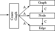
Figure 11.8 Class Graph aggregates objects of type Node and class Node aggregates objects of type Edge. Class CreateGraph reads node and edge data from a file and creates an object of type Graph. “C” indicates the “aggregation” relation which is also known as the “composite,” relation. “A” indicates the association relation.

11.5.2  Comparing integration strategies

Each of the integration strategies discussed above has their pros and cons as examined in the following:

1. Stubs and drivers: Other than the big-bang strategy, all require the creation of either stubs or drivers, or both. Thus, top-down integration requires the creation of stubs for components at the lower level. On the other hand the bottom-up integration strategy requires the creation of drivers. As discussed earlier, design of both stubs and drivers could be challenging and costly. Thus, neither strategy seems to have any advantage over the other when viewed from the point of view of stub or driver creation. Certainly, depending on the specific project, it might be easier to create stubs than drivers, or vice versa. In that case one strategy might be preferred over the other.
   
   

   Top-down integration requires the creation of stubs while bottom-up integration requires the creation of drivers.

2. Partially working program: There are situations when the management wishes to demonstrate a system to a select group of potential customers. Top-down approach has the advantage that one could have a partially working system, also known as a skeleton system, before integration testing is complete. Bottom-up approach builds the system from the bottom and hence a working system is not available until the top level components have been integrated. In most modern systems that use a graphical user interface (GUI), it might be best to begin integration into the GUI. Doing so would ensure that a skeletal system is always available regardless of whether the top-down or the bottom-up approach is used.
3. Error location: Prior to integration testing, one usually would not know the location of integration errors. However, based on past experience and skills of the development teams, as well as various software metrics, one might be able to flag components likely to be more erroneous than others.

11.5.3  Specific stubs and retesting

As mentioned earlier, a stub for class C2 is needed when class C1 depends on C2 and C2 is not available when testing C1. A stub is a temporary replacement for a class and hence it should be easy to write and test a stub. Obviously, this implies that a stub will perform simple tasks like always returning a fixed or a random data when requested rather than actually executing code to generate data as per the requirements. This simplicity might not allow for a thorough testing of C1. In any case, stubbing a class has an associated cost. Hence the cost ought to be a consideration when deciding which classes to stub when there is a choice.

 

When C1 depends on class C2 we say that C1 is a client of C2. In this case C2 is considered as a server class. Of course, it is possible that C1 and C2 depend on each other in which case both serve as client and server classes for each other. The stub for a server class depends on the requirements placed by its client. Thus, two stubs might be required for a single server class if it serves two clients. Such stubs are known as specific stubs. Each specific stub is written to simulate a simplified behavior of a server class so as to fulfill the testing needs of the corresponding client class.

 

The client class needs to be retested when the code for a stubbed class is tested. However, this retesting is limited to the edges that connect the client to the stubbed class. For example, if the only dependence between C1 and C2 is a method m in server class C2 that is called by C1, then retesting of C1 needs to focus only on the calls to m. Doing so reduces the test cases that are rerun during a retest. Nevertheless, retesting has an associated cost. Thus, when deciding which classes to stub, or not to stub, one needs to consider the cost of retesting. In cases where the dependence between two classes is significant, and there exists a cycle involving the two, it might be best to test the two together rather than test them incrementally.

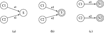
Example 11.6   Figure 11.9(a) shows two client classes C1 and C2 that depend on server class S. If S is not available while testing C1 or C2, a stub for S is needed as shown in Figure 11.9(b). However, to keep the stub simple, one may decide to create two specific stubs S1 and S2 as shown in Figure 11.9(c). In either case, when class S is available, C1 needs to be retested with respect to edge e1. Similarly, class C2 needs to be tested with respect to edge e2.

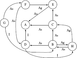
Example 11.7   Consider the ORD in Figure 11.10. Note that this ORD contains a cycle between nodes B and H. Hence at least one stub is needed for incremental testing. Now consider the following test sequence: A, E, C, F using STUB(F, D), H using STUB(H, B), D, B, and G. In this sequence two specific stubs are needed as there is one client of each server class D and F needed by their respective client classes F and H. Now suppose it is decided to minimize the number of specific stubs. This could be done by using only one stub class B and the following test sequence: A, E, C, H using STUB(H, B), D, F, B, G.

 

An ORD might have a cycle. In this situation at least one stub is needed if pure incremental testing is preferred.

Figure 11.9 (a) Client classes C1 and C2 and server class S. (b) Server classes S stubbed. (c) Specific stubs S1 and S2 for server class S.

Figure 11.10 A sample ORD with eight classes containing cycles between classes B, H.

In the above test sequences the number of specific stubs is the same as the number of stubs. However, this is not always true as is shown later when we look at the algorithms for generating a test sequence. Also see Exercise 11.8.

The cost of retesting and stubbing is class and project dependent and hence it is difficult to offer any specific rules to decide whether or not to stub a class when dependence exists. The algorithms that follow attempt to minimize the number of stubs and the associated costs of stubbing and retesting.

The TD and the TJJM methods that follow focus on minimizing the stub count while the BLW method aims to minimize the cost of retesting and stubbing of server classes. Note that none of these methods claims to generate an optimal set of stubs. Also, as mentioned above, minimizing the number of stubs for incremental testing does not necessarily mean minimizing the cost of integration testing. Thus, even though the three methods described below are useful in practice, the outcome might need to be subjected to further project and code dependent considerations before the final decision is made by the test team on what or what not to stub.

 

11.6  Finding a Near-Optimal Test Order

The problem of finding an optimal integration sequence is NP-complete. Thus, several methods have been proposed to find a near-optimal integration sequence. Three such methods are introduced in the following sections. These are referred to as the Tai-Daniels (TD), Traon-Jéron-Jézéquel-Morel (TJJM), and Briand-Labiche-Wang (BLW) methods. Each of the methods described below takes an ORD as input in the form of a directed graph. It is assumed that each edge in the ORD is labeled by exactly one relationship, i.e. I, Ag, and As. Thus, in the event a class Y is associated with class X by both the I and As relations, it is best to use the As relation in the input ORD. A comparison of the three methods is given after each has been examined.

 

11.6.1  The TD method

The TD method takes an ORD G as input and applies the following sequence of steps to generate an integration sequence.

 

Step A	Assign major level numbers 1, 2, 3, and so on to each node in G. The assignment of major levels partitions the nodes in the ORD into n categories, where n ≥ 1 is the number of major levels. Nodes at major level 1 do not have any outgoing inheritance or aggregation edges. Nodes at major level 2 have inheritance or aggregation edges to nodes at level 1. In general, each node at major level i, 1 < i ≤ n, has an inheritance or an aggregation edge to nodes at major level j < i and at least one such edge to a node at major level (i – 1). Once partitioned in this way, the classes at major level i are considered for testing prior to those at major levels k, k > i. The order in which classes at major level i are to be tested is determined in the next step. A procedure named assignMajorLevels for assigning major level to each node in G discussed in the next page.
Step B	Assign minor level numbers 1, 2, 3, and so on to each node in G. Note from the previous step that each major level has one or more nodes from G. A minor level is assigned to each node to decide the sequence in which the nodes at a major level are to be tested. Procedure assignMinorLevel. This procedure aims at assigning minor levels to nodes with the goal of minimizing the stubs needed for integration testing.
Step C	Generate test sequence, stubs, and retest edges. Once the major and minor levels have been assigned, each node has two integers (i, j) associated with it, where i denotes its major level and j its minor level. Testing begins with nodes at major level 1. Among the nodes at major level 1, nodes at minor level 1 are tested first, followed by the nodes at minor level 2, and so on. Nodes at a major level with the same minor levels can be tested concurrently. Once the nodes at major level 1 have been tested, nodes at major level 2 are considered for testing, and so on. Note that testing a node A at major level i requires a stub for a node B that has an incoming association edge from A and is at a higher level, major or minor, than A. Also, while testing a node A, any edge to a node at a lower level, major or minor, needs to to be retested.

 

The following subsections describe the procedures corresponding to the three steps mentioned above. However, prior to going through the procedures mentioned below, you may view Figure 11.12 in case you are curious to know how an ORD looks like after its nodes have been assigned major and minor levels.

A. Assign major level numbers

Each node in an ORD G is assigned a major level number. A level number is an integer equal to or greater than 1. The purpose of assigning level numbers will be clear when we discuss Step 3 of the method. The assignment of major level numbers to each node in G is carried out using a depth first search while ignoring the association edges to avoid cycles.

 

The algorithm for assigning major level numbers as described next consists of two procedures. Procedure assignMajorLevel marks all nodes in the input ORD as “not visited.” Then, for each node that is not visited yet it calls procedure levelAssign. The levelAssign procedure does a depth first search in the ORD starting at the input node. A node that has no successors is assigned a suitable major level number starting with 1. If node n₁ is the immediate ancestor of node n₂ then n₁ will be assigned a level one greater than the level of n₂.

Procedure for assigning major level numbers.

Input:	An ORD G.
Output:	ORD G with major level number (≥ 1) assigned to each node.

Procedure: assignMajorLevel

/*	N denotes the set of all nodes in G. The major level number of each node is initially set to 0. maxMajorLevel denotes the maximum major level number assigned to any node and is initially set to 0. The association edges are ignored when applying the steps below.
*/

Step 1	Mark each node in N as “not visited.”
Step 2	Set level = major.
Step 3	For each node n ∈ N marked as “not visited” apply the levelAssign procedure. A node that is visited has already been assigned a major level number other than 0.
Step 4	Return G.

End of Procedure assignMajorLevel

 

Procedure for assigning a level number (major or minor) to a node.

Input:	(a) An ORD G. (b) A node n ∈ G. (c) level.
Output:	G with major or minor level number assigned to node n depending on whether level is set to major or minor, respectively.
Procedure:	levelAssign

/*	This procedure assigns a major or minor level number to the input node n. It does so using a recursive depth first search in G starting at node n.
*/

Step 1	Mark n as “visited.”
Step 2	Let Sn = successor nodes of n.
Step 3	if (Sn = Ø) then assign 1 to n as its major or minor level depending on level and return.
Step 4	if (S ≠ Ø) then for each node m ∈ S do the following:
4.1	if (m is not visited) then apply levelAssign to m.
4.2	Set maxLevel = maximum major (minor) level among all nodes in Sn + 1.
4.3	if (maxMajorMinorLevel < maxLevel) then maxMajor-MinorLevel=maxLevel.
Step 5	Return G.

 

End of Procedure levelAssign

Example 11.8   Let us now apply procedure assignMajorLevel to the graph G in Figure 11.11(b) and assign major levels to each node in the graph. The set of nodes N = {A, B, C, D, E, F, G, H}. In accordance with Step 1, begin by marking all nodes in N to “not visited.” As no node has been assigned a major level, set maxMajorLevel=0. A node is indicated as “not visited” by adding a superscript n to its name. Thus, Aⁿ indicates that node A is not visited. Also, the successors of node X are denoted as S_X.

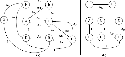
Figure 11.11 (a) An ORD consisting of nodes (classes) labeled A through H. This ORD contains three inheritance edges labeled I, 11 association edges labeled A, and three aggregation edges labeled Ag. (b) ORD in (a) without the association edges. This is used to illustrate the TD method.

Now move to Step 3. Let us start with node Aⁿ. As this node is not visited, enter procedure levelAssign. The ensuing steps are described below.

levelAssign.Step 1: Mark node Aⁿ as visited.

levelAssign.Step 2: As node A has no successors, S_A = Ø.

levelAssign.Step 3: Assign major level 1 to A and return from levelAssign.

assignMajorLevel.Step 3: Select the next node in N. Let this be node Bⁿ.

levelAssign.Step 1: Mark Bⁿ as visited.

levelAssign.Step 2: Get the successor set for node B. Thus, S_B ={Hⁿ}.

levelAssign.Step 4: Select the next node in S_B, which is Hⁿ.

levelAssign.Step 1: This is a recursive step. Mark Hⁿ to visited.

levelAssign.Step 2: Get the successors of H. S_H = {Cⁿ}.

levelAssign.Step 4: Select the next node in S_H, which is Cⁿ.

levelAssign.Step 1: As Cⁿ is not visited we apply levelAssign to this node.

levelAssign.Step 1: Mark node Cⁿ as visited.

levelAssign.Step 2: As node C has no successors, S = Ø.

levelAssign.Step 3: Assign major level 1 to C and return from levelAssign.

levelAssign.Step 2: Set level=maxMajorLevel + 1 = 2.

levelAssign.Step 3: Assign major level 2 to H. Return from levelAssign.

The remaining steps are left to the reader as an exercise. At the end of procedure assignMajorLevel the following major level numbers are assigned to the nodes in G.

Major level 1 assigned to nodes A, E, and C.

Major level 2 assigned to nodes F and H.

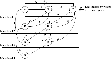
Figure 11.12 Graph G from Figure 11.11(a) with major and minor levels assigned. Nodes at the same major levels are placed just above the corresponding horizontal line. Minor level numbers are placed just above each node. Edge deletion is explained in Example 11.9.

Major level 3 assigned to nodes D and B.

Major level 4 assigned to node G.

Figure 11.12 shows graph G with the major levels assigned.

 

B. Assign minor level numbers

In this step minor level numbers are assigned to each node. Assignment of minor level numbers is done for nodes within each major level. Thus, nodes at major level 1 are processed first, followed by nodes at the next higher major level, and so on. Of course, the processing of nodes at different major levels is independent and hence which set of nodes is assigned minor level numbers does not in any way affect the resulting assignment. The procedure for assigning minor level numbers follows.

 

Procedure for assigning minor level numbers.

Inputs:	(a) An ORD G with minor level numbers assigned to each node. (b) maxMajorLevel that denotes the maximum major level assigned by Procedure assignMajorLevel.
Output:	ORD G with minor level numbers assigned to each node in G.

 

Procedure: assignMinorLevel

Perform the following steps for each major level i, 1 ≤ i ≤ maxMajorLevel.

 

Step 1	Let Ni be the set of all nodes at major level i. if (|Ni| = 1) then assign 1 as the minor level to the only node in Ni else move to the next step.
Step 2	if (nodes in Ni do not form any cycle) then assign minor level numbers to the nodes in Ni using procedure assignMinorLevelNumbers.
Step 3	Break cycles by applying procedure breakCycles.
Step 4	Use procedure assignMinorLevelNumbers to assign minor level numbers to the nodes in Ni.
Step 5	Return G.

 

End of Procedure assignMinorLevel

 

At Step 2 in Procedure assignMinorLevel we need to determine all strongly connected components in G′. This can be done by applying, for example, Tarjan’s algorithm to the nodes at a major level. The strongly connected components are then used to determine whether or not a cycle exists. Tarjan’s algorithm is not described in this book but see the Bibliographic Notes section for a reference.

 

Procedure breakCycles is called when there exist one or more cycles among the nodes at a major level. Recall that cycles among a set of nodes might be formed due to the existence of association edges among them. The breakCycles procedure takes a set of nodes that form a cycle as input and breaks all cycles by suitably selecting and removing association edges. Cycles are first broken by removing edges ensuring that a minimum number of stubs is needed. However, doing so might not break all cycles. Thus, if cycles remain, additional association edges are removed using edge weight as the criterion as explained in the procedure below.

 

Procedure for breaking cycles in a subgraph of an ORD.

Inputs:	(a) A subgraph G′ of ORD G that contains one or more cycles and of which all nodes are at the same major level. (b) Integer m, where 1 ≤ m ≤ maxMajorLevel, is the major level of the nodes in G′.
Output:	Modified G′ obtained by the removal of zero or more edges from the input subgraph.

Procedure: breakCycles

Step 1	Let X ∈ G′ be a node such that there is an association edge to X from a node at a major level lower than m. Let S denote the set of all such nodes. Note that if a node X in G′ has an association edge coming into it from a node at a lower major level then there already exists a stub for X because all nodes at major level less than m are tested prior to testing the nodes at level m.
Step 2	if (S is non-empty) then construct E as the set of all association edges from nodes in G′ that are incident at nodes in S else go to Step 5.
Step 3	if (E is non-empty) then remove all edges in E from G′ .
Step 4	if (G′ contains no cycles) then return else move to the next step.
Step 5	Compute the weight of each edge in G′ that has not been deleted. Let n1 be the source and n2 the destination node of an edge e. Then the weight of e is s + d, where s is the number of edges incident upon n1 and d is the number of outgoing edges from n2.
Step 6	Let Es = {e1, e2,…, en} be a list of all undeleted edges in G′ sorted in the decreasing order of their weights. Thus, the weight of e1 is greater than or equal to that of e2, that of e2 is greater than or equal to the weight of e3, and so on. Delete from G′ the edges in Es one by one starting with e1. Continue the process until no cycles remain in G′.
Step 7	Return G′ .

End of Procedure breakCycles

 

The next procedure assigns minor level numbers to all nodes at a major level given that they do not form a cycle. This procedure is similar to procedure assignMajorLevel. It takes a subgraph G′ of the original ORD G as input. G′ has no cycles. It begins by marking all nodes in G′ to “not visited.” It then sets level to minor and calls procedure levelAssign to assign the minor level numbers to each node in G′.

Procedure for assigning minor level numbers to nodes at a major level.

 

Input:	Subgraph G′ of G with no cycles.
Output:	G′ with minor level numbers assigned to each node.

 

Procedure: assignMinorLevelNumbers

 

Step 1	Mark each node in G′ as “not visited.”
Step 2	Set level=minor.
Step 3	For each node n ∈ G′ marked as “not visited” apply the levelAssign procedure. A node that is visited has already been assigned a minor level number other than 0.

 

End of Procedure assignMinorLevelNumbers

Example 11.9   Let us now assign minor level numbers to the ORD G in Figure 11.11(a). The major level numbers have already been assigned to the nodes and are shown in Figure 11.12. Begin by applying Procedure assignMinorLevel.

assignMinorLevel. Let i= 1. Thus, the first set of nodes to be processed are at major level 1.

assignMinorLevel.Step 1: N₁ = {A, C, E}. As N₁ has more than one node, we move to the next step.

assignMinorLevel.Step 2: As can be observed from Figure 11.12, N₁ has one strongly connected component consisting of nodes A, C, and E. This component has a cycle. Hence move to the next step with the subgraph of G′ of G consisting of the nodes in N₁, and major level m = 1.

breakCycles.Step 1: As all nodes in G′ are at major level 1, we get S = Ø.

breakCycles.Step 2: S is empty hence move to Step 5.

breakCycles.Step 5: The weight of each of the four edges in G′ is computed as follows: A – C = 2 + 2 = 4; C – E = 1 + 1 = 2; E – A = 1 + 1 = 2: and C – A = 1 + 1 = 2.

breakCycles.Step 6: Es= {A – C, C – E, E – A, C – A}. The first edge to be deleted is A – C as it has the highest weight. As should be evident from Figure 11.12 doing so removes the cycles in G′. Hence there is no need to delete additional edges.

assignMinorLevel.Step 4: Now that the only cycle in G′ is removed, the minor level numbers can be assigned.

assignMinorLevelNumbers.Step 1: Mark all nodes in G′ as “not visited.”

assignMinorLevelNumbers.Step 2: level=minor.

assignMinorLevelNumbers.Step 3: We need to loop through all nodes in G′ that are marked as “not visited.” Let us select node A.

levelAssign.Step 1: Node Aⁿ is marked as “visited.”

levelAssign.Step 2: As the edge A – C has been deleted, A has no successors. Thus, S = Ø.

levelAssign.Step 3: Assign 1 as the minor level to node A.

The remainder of this example is left to the reader as an exercise. Moving forward, nodes E and C are assigned, respectively, minor levels 2 and 3. Next, nodes at major level 2 are processed as described above. This is followed by nodes at major levels 3 and 4. Note that there are no cycles among the strongly connected components at major levels 2, 3, and 4 and hence no edges need to be deleted. Figure 11.12 shows the final assignment of major and minor levels to all nodes in ORD G. Also indicated in this figure is the edge A – C deleted by using the edge-weight criterion.

 

C. Generate test sequence, stubs, and retest edges

Let us now look into how the test sequence, stubs, and edges to be retested are generated. As mentioned earlier, the basic idea is to test all nodes at major level 1, followed by those at major level 2, and so on. Doing so may require one or more stubs when a node at major level i has dependency on a node at a major or minor level j, i ≤ j. Procedure generateTestSequence generates the test sequence from an ORD G in which each node has been assigned a major and a minor level. The procedure also generates a list of nodes that ought to be stubbed and a set of edges that need to be retested.

 

Procedure for generating test and retest sequence.

Inputs:	(a) ORD G with major and minor level numbers assigned. (b) maxMajorLevel. (c) maxMinorLeve [i] for each major level 1 ≤ i ≤ maxMajorLevel.
Outputs:	(a) TestSequence, (b) stubs, and (c) edges to be retested.
Procedure:	generateTestSequence

 

Step 1	Let testSeq, stubs, and retest denote, respectively, the sequence in which nodes in G are to be tested, a list of stubs, and a list of edges to be retested. Initialize testSeq, stubs, and retest to empty.
Step 2	Execute the following steps until Step 2.1.9 for 1 ≤ i ≤ maxMajorLevel.
2.1	Execute the following steps until Step 2.1.9 for minor level j, 1 ≤ j ≤ maxMinorLevel[i].
2.1.1	Let IT be the set of nodes at major level i and minor level j that are connected by an association edge. Note that these nodes are to be tested together. If there are no such nodes then IT = {n}, where n is the sole node at level(i, j).
2.1.2	Update test sequence generated so far. testSequence = testSequence+IT.
2.1.3	Let N be the set of nodes at major level i and minor level j.
2.1.4	For each node n ∈ N, let SMajorn be the set of nodes in G at majorlevel greater than i, i < maxMajorLevel, such that there is an association edge from n to each node in SMajor. Such an edge implies the dependence of n on each node in SMajor. SMajorn = Ø for i = maxMajorLevel.
2.1.5	For each node n ∈ N, let SMinorn be the set of nodes in G at minor level greater than j, j < maxMinorLevel[i], such that there is an association edge from n to each node in SMinor. SMinorn = Ø for j = maxMinorLevel[i].
2.1.6	Update the list of stubs generated so far.stubs= stubs+SMajorn +SMinorn for each n ∈ N.
2.1.7	For each node n ∈ N, let RMajorn be the set of nodes in G at major level less than i, i < maxMajorLevel, such that there is an edge to n from a node in RMajor. RetestMajorn = Ø for i = maxMajorLevel. Let REMajor be the set of edges to node n from each node in RMajor.
2.1.8	For each node n ∈ N, let RMinorn be the set of nodes in G at minor level less than j, j < maxMinorLevel[i], such that there is an edge to n from a node in RMinor. RMinorn = Ø for j = maxMinorLevel[i]. Let REMinor be the set of edges to node n from each node in Minor.
2.1.9	Update the list of retest edges. retest= retest+ REMajorn+ REMinorn for each n ∈ N .
Step 3	Return testSequence, stubs, and retest.

 

End of Procedure generateTestSequence

Example 11.10   Let us now apply Procedure generateTest Sequence to the ORD in Figure 11.12.

genTestSequence.Step 1: testSeq= Ø, stubs= Ø, and retest=Ø.

genTestSequence.Step 2: Set next major level i= 1.

genTestSequence.Step 2.1: Set next minor level j= 1.

genTestSequence.Step 2.1.1: Get nodes at major level 1 and minor level 1. IT = {A}.

genTestSequence.Step 2.1.2: testSeq = {A}.

genTestSequence.Step 2.1.3: N = {A}. A is the only node at major level 1 and minor level 1.

genTestSequence.Step 2.1.4: SMajor_c.

genTestSequence.Step 2.1.5: SMinor = Ø.

genTestSequence.Step 2.1.6: stubs = {C}.

genTestSequence.Step 2.1.7: RMajor_A = {}. REMajor_A = {}.

genTestSequence.Step 2.1.8: REMajor_A = {}. REMajor_A = {}.

genTestSequence.Step 2.1.9: No change in retest.

genTestSequence.Step 2.1: Set next minor level j = 2.

genTestSequence.Step 2.1.1: Get nodes at major level 1 and minor level 2. IT = {E}.

genTestSequence.Step 2.1.2: testSeq = {A, E}.

genTestSequence.Step 2.1.3: N= {E}.

genTestSequence.Step 2.1.4: SMajor_E = {F}.

genTestSequence.Step 2.1.5: SMinor_E = Ø.

genTestSequence.Step 2.1.6: stubs = {C, F}.

genTestSequence.Step 2.1.7: RMajor_E = Ø. REMajor_E = Ø.

genTestSequence.Step 2.1.8: RMinor_E = Ø. REMinor_E = Ø.

genTestSequence.Step 2.1.9: No change in retest.

genTestSequence.Step 2.1: Set next minor level j = 3.

genTestSequence.Step 2.1.1: Get nodes at major level 1 and minor level 3. IT = {C}.

genTestSequence.Step 2.1.2: testSeq = {A, E, C}.

genTestSequence.Step 2.1.3: N = {C}. C is the only node at major level 1 and minor level 1.

genTestSequence.Step 2.1.4: SMajor_C = {H}.

genTestSequence.Step 2.1.5: SMinor_C = Ø.

genTestSequence.Step 2.1.6: stubs = {C, F, H}.

genTestSequence.Step 2.1.7: RMajor_C = Ø. REMajor_C = Ø.

genTestSequence.Step 2.1.8: RMinor_C = Ø. REMinor_C = Ø = {A–C}.

genTestSequence.Step 2.1.9: retest = {A–C}. This implies that when testing class C, the association edge A–C needs to be retested because A was tested with a stub of C and not the class C itself.

The remainder of this example is left as an exercise for the reader to complete. The final class test sequence is as follows:

A → E → C → F → H → D → B → G

The following stubs are needed:

Stub for C used by A

Stub for F used by E

Stub for H used by C

Stub for D used by F

Stub for B used by H

The following edges must be retested:

When testing C retest A–C.

When testing F retest E–F.

When testing H retest C–H.

When testing D retest F–D.

When testing B retest H–B.

11.6.2  The TJJM method

The TJJM method uses a significantly different approach than the TD algorithm for the determination of stubs. First, it does not distinguish between the types of dependance. Thus, the edges in the ORD input to the TJJM algorithm are not labeled. Second, it uses Tarjan’s algorithm recursively to break cycles until no cycles remain. Third, while breaking a cycle, the weight associated with each node is computed differently as described below. Following are the key steps used in the TJJM algorithm starting with an ORD G.

 

Step A	Find the strongly connect components (SCCs) in G. Suppose n > 0 SCCs are obtained. Each node in an SCC has an index associated with it indicating the sequence in which it was traversed while traversing the nodes in G to find the SCCs. An SCC with no cycles is considered trivial. Only non-trivial SCCs are considered in the following steps. Tarjan’s algorithm can be applied to find the SCCs in G.
Step B	For each non-trivial SCC s found in the previous step, and for each node k in s, identify edges that are coming into k from its descendants within s. A node m is a descendant of node k if the traversal index of m is greater than that of node k implying that node m was traversed after node k. All such edges are known as frond edges.
Step C	For each non-trivial SCC, compute the weight of each node as the sum of the number of incoming and outgoing frond edges.
Step D	In each non-trivial SCC select the node with the highest weight as the root of that SCC. Remove all edges coming into the selected root. The selected node is also marked as a stub.
Step E	In this recursive step, for each non-trivial SCC s, set G = s and apply this method starting from Step A.

 

The above algorithm terminates when all SCCs to be processed in the steps following Step A are non-trivial. Upon termination of the algorithm one obtains one or more directed acyclic graphs consisting of nodes (classes) in G. Topological sort is now applied to each DAG to obtain the test order for the classes.

Procedure for generating stubs and test order.

 

Inputs:	(a) ORD G and (b) Stubs.
Outputs:	(a) Stubs and (b) Modified G with no cycles.

 

Procedure: TJJM

 

Step 1	Find the set S of non-trivial strongly connected components in G. A non-trivial component is one with no cycles. Each node in G is assigned a unique traversal index. This index is an integer, starting at 1, that denotes the sequence in which the node was traversed while finding the strongly connected components. For any two nodes n and m in a component s ∈ S, n is considered an ancestor of m if its traversal index is smaller than that of m.
Step 2	Return if S is empty. Otherwise, for each component s ∈ S, do the following:
2.1	For each node n ∈ s identify edges entering n from its descendants in s. Such edges are known as a frond edges.
2.2	For each node n ∈ s compute the weight of n as the sum of the number of incoming and outgoing frond edges.
2.3	Let m ∈ s be the node with the highest weight. Stubs = Stubs ∪ {m}. In case there are multiple nodes with the same highest weight, select one arbitrarily. Delete all edges entering m from within s. This step breaks cycles in s. However, some cycles may remain.
2.4	Set G = s and apply procedure TJJM. Note that this is a recursive step.

End of Procedure TJJM

 

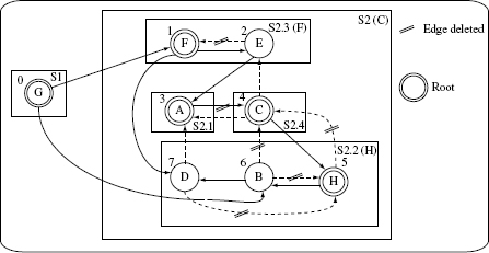
Figure 11.13 Strongly connected components found by applying the TJJM algorithm to the ORD in Figure 11.11. Nodes with two circles are selected roots of an SCC. Each SCC is enclosed inside a rectangle and labeled as Sx (y), where x denotes the SCC number, and when indicated, y denotes the node selected as a root for recursive application to break further cycles. Traversal sequence index is placed against the corresponding node.

Example 11.11   Let us apply the above mentioned steps to the ORD in Figure 11.11. This ORD has 8 nodes and 17 edges.

 

Step 1	The first application of Tarjan’s algorithm as in Step A leads to two SCCs labeled S1 and S2 and enclosed inside a rounded rectangle in Figure 11.13. SCC S1 is trivial as it contains only one node. SCC S2 contains the remaining seven nodes and has several cycles. The traversal index of each node is placed next to the node label. For example, the traversal index of node F is 1 and that of node B is 6. Thus we have S = {S2}.
Step 2	Set s = S2 and move to the next step.
Step 2.1	Frond edges are shown as dashed lines in Figure 11.13. For example, node C has two incoming and two outgoing frond edges. The incoming frond edges are from nodes B and H as these two nodes are descendants of C. The outgoing frond edges are to nodes A and E as both these nodes reancestors of node C.
Step 2.2	Using the frond edges shown in Figure 11.13, we obtain the following weights: F: 1; A, B and E: 2; H: 3; and C: 4.
Step 2.3	Node C has the highest weight and hence is selected as the root of SCC S2. This node has three incoming edges A–C, B–C and H–C which are deleted as shown in Figure 11.13. Stubs = Stubs ∪{C}.
Step 2.4	Set G = S2 and execute procedure TJJM.
Step 1	Four SCCs are obtained labeled in Figure 11.13 as S2.1, S2.2, S2.3, and S2.4. Of these, S2.1 and S2.4 are trivial and hence not considered further. Thus, S = {S2.2, S2.3}.
Step 2	Set s = S2.2.
Step 2.1	As in Figure 11.13, edges B–H and D are the two fronds s.
Step 2.2	The weights of various nodes are: nodes B and D: 1 and node H: 2.
Step 2.3	Node H is selected as the root of S2.2. Stubs = Stubs ∪{H}. Edges B–H and D–H are deleted as these are incident on node H.
Step 2.4	Set G = S2.2 and execute procedure TJJM.
Step 1	There are three SCCs in S2.2. Each of these is trivial and consists of, respectively, nodes D, B, and H. Thus, S = Ø. Return from this execution of TJJM.
Step 2	Set s = S2.3.
Step 1	In S2.3 there is one frond edge, namely, E–F.
Step 2.3	The weight of each node in S2.3 is 1.
Step 2.3	As both nodes in S2.3 have the same weight, either can be selected as the root. Let us select node F as the root. Stubs = Stubs ∪{F)
Step 2.4	Set G = S2.3 and apply TJJM.
Step 1	There are two SCCs in the modified S2.3. Each of these is trivial and consists of, respectively, nodes E and F. Hence return from this call to TJJM.

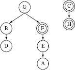
Figure 11.14 DAGs obtained after deleting edge indicated in Figure 11.13.

There are no remaining non-trivial SCCs. Hence the algorithm terminates. We obtain Stubs = {C, F, H}. Figure 11.14 shows the DAG obtained after having removed the edges from the ORD in Figure 11.13 as described above. Applying topological sort first to the DAG rooted at G and then to the DAG rooted at C gives the following test sequence:

1. Test A using Stub(C)
2. Test E using Stub(F) and A
3. Test D using A and Stub(H)
4. Test F using E and D
5. Test B using Stub(C), D, and Stub(H)
6. Test G using F and B
7. Test H using B and Stub(C)
8. Test C using A, H, and E

It may be noted that the stubs created by applying the TJJM algorithm depend on the sequence in which the nodes are traversed when identifying the SCCs in Step 1. Exercise 11.9 asks for applying the algorithm with a different traversal order than used in Example 11.11.

 

Stubs created by the TJJM algorithm depend on the sequence in which the nodes are traversed. Hence, the generated set of stubs is not unique.

11.6.3  The BLW method

The BLW method aims to minimize the number of specific stubs. As explained in Section 11.5.3, minimizing specific stubs will likely reduce the total cost of integration testing by allowing the construction of simpler stubs, one for each client.

The BLW method is similar to the TJJM method in that it recursively computes SCCs and breaks cycles by removing edges. However, the strategy to remove cycles from an SCC differentiates it from the TJJM method. Recall that the TJJM method uses the following steps to break cycles in a non-trivial SCC:

 

1. Compute the weight of each node in the SCC as the sum of the incoming and outgoing frond edges.
2. Identify the node with the highest weight as the new root, and a stub, of the SCC.
3. Delete all edges coming into the root node from within the SCC. 

Instead, the BLW method uses the following steps to identify and remove edges from an SCC:

1. Compute the weight of each association edge X–Y in the SCC as the product of the number of edges entering node X and the number of edges exiting node Y. Note that in contrast to the TJJM method, this step does not use the notion of fronds. Also, in this step the weight of an edge, not a node, is computed.
   
   

   The BLW method does make use of the edge labels in an ORD.

2. Delete the edge with the highest weight. In case there are multiple such edges, select any one. If the edge deleted is X–Y, then node Y is marked as a stub. The specific stub in this case is Stub(X, Y). Thus, instead of deleting all edges entering a selected node, only one edge is removed in this step. Note that only association edges are deleted. Again, this is in contrast to the TJJM method which could delete any type of edge. 

All steps in the BLW algorithm are the same as shown in Procedure TJJM. The BLW algorithm makes use of ideas from the TD and TJJM methods. From the TD method it borrows the idea of computing edge weights. From the TJJM method it borrows the idea of recursively computing the SCCs and deleting one association edge at a time. By doing so the BLW method gets the following advantages:

1. It creates all the stubs needed. This is unlike the TD method that may force the combined testing of some classes.
2. By aiming at reducing the number of specific stubs, it attempts to reduce the cost of an integration test order.

The following procedure is used in the BLW method for generating stubs. The test order and specific stubs can be determined from the resulting DAG and the stubs.

 

Inputs:	(a) ORD G and (b) Stubs.
Outputs:	(a) Stubs and (b) modified G with no cycles.

Procedure: BLW

Step 1	Find the set S of non-trivial strongly connected components in G. A non-trivial component is one with no cycles.
Step 2	Return if S is empty. Otherwise, for each component s ∈ S, do the following
2.1	For each association edge X – Y ∈ s compute its weight as the product of the number of edges entering node X and the number of edges exiting node Y from within s.
2.2	Let X – Y ∈ s be the edge with the highest weight. Remove X–Y from s. Set Stubs = Stubs ∪ {Y}. In case there are multiple edges with the same highest weight, select one arbitrarily.
2.3	Set G = s and apply procedure BLW. Note that this is a recursive step. End of Procedure BLW

Procedure BLW is illustrated next with an example to find the stubs in the ORD in Figure 11.11.

Example 11.12   Let us apply procedure BLW to the ORD in Figure 11.11.

 

Step 1	The first application of Tarjan’s algorithm as in Step A gives us two SCCs. The non-trivial SCC labeled S1 is shown in Figure 11.15. Thus we have S = {S1}. There is only one trivial SCC in this case that consists of node G.
Step 2	Set s = S1.
Step 2.1	The weights of various edges in s are as follows:
Step 2.2	The underlined edges H–B and A–C have the highest weights. H–B is arbitrarily selected and removed from s. Hence, node B is marked as a stub. Stubs = Stubs ∪ {B}.
Step 2.3	Set G = s and execute procedure BLW.

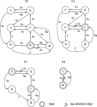
Figure 11.15 SCCs, deleted edges, and stubs obtained by applying the BLW algorithm to the ORD in Figure 11.13. Only the non-trivial SCCs, i.e., those with one or more cycles, are shown.

Step 1	We get two SCCs only one of which is non-trivial and is labeled S2 in Figure 11.15. The trivial SCC consists of only node B.
Step 2	Set s = S1.
Step 2.1	The weights of various edges in s are as follows:
Step 2.2	Edge A–C has the highest weight and is removed from s. Hence, node C is marked as a stub. Stubs = Stubs ∪ {C}.
Step 2.3	Set G = s and execute procedure BLW.
Step 1	Once again we get two SCCs only one of which is non-trivial and is shown as S3 in Figure 11.15. The trivial SCC consists of the lone node A.
Step 2	Set s = S3.
Step 2.1	The weights of various edges in s are as follows:
Step 2.2	Edge E–F has the highest weight and is removed from s. Hence, node F is marked as a stub. Stubs = Stubs ∪ {F}.
Step 2.3	Set G = s and execute procedure BLW.
Step 1	We get four SCCs only one of which is non-trivial and is labeled S4 in Figure 11.15. The trivial SCCs are {E}, {D}, and {F}.
Step 2	Set s = S4.
Step 2.1	The weight of the lone edge C–H in s is (1*1)=1.
Step 2.2	Edge C–H obviously has the highest weight and is removed from s. Hence, node H is marked as a stub. Stubs = Stubs ∪{F}.
Step 2.3	Set G = s and execute procedure BLW.

The algorithm will now terminate after returning from various recursive calls as there are no remaining non-trivial SCCs. The DAG obtained after deleting the edges as above is shown in Figure 11.16. The DAG, together with the class relationships in Figure 11.11, can now be traversed to obtain the following test order:

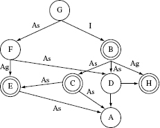
Figure 11.16 DAG obtained by applying procedure BLW to the ORD in Figure 11.11.

1. Test A using Stub(C)
2. Test E using Stub(F) and A
3. Test C using A, Stub(H), and E
4. Test H using Stub(B) and C
5. Test D using A and H
6. Test F using E and D
7. Test B using C, D, and H
8. Test G using F and B

A total of four specific stubs are needed. These are Stub(C, A), Stub(F, A), Stub(H, E), and Stub(B, C).

11.6.4  Comparison of TD, TJJM, and the BLW methods

Two criteria are useful in comparing the utility and effectiveness of the methods for generating a test order. First criterion is the number of stubs and specific stubs needed. As mentioned earlier, the cost of integration testing is proportional to the number of specific stubs needed and hence this seems to be a reasonable criterion. The second criterion is the time required to generate the test order given an ORD.

 

Several ORDs are used to compare the different methods for test order generation using the criteria mentioned above. Some of these ORDs are from the literature on integration testing while others were generated randomly as described next.

Generating a random ORD: Table 11.1 lists three sets of ORDs used for comparing TD, TJJM, and BLW. The first set of three ORDs, labeled TDG, TJJMG, and BLWG, are from the publications where they were first reported. The second set of four ORDs are derived randomly and so are the ORDs in the third set. ORDs in Set 2 are relatively small, each consisting of 15 classes. Those in Set 3 are relatively large, each consisting of 100 classes.

 

The generation process ensures that a randomly generated ORD has no cycle involving the inheritance and aggregation edges. Also, the generated ORDs do not have multiple inheritance. Each randomly generated ORD has the following parameters:

 

• number of nodes (n),
• density (between 0 and 1), where 0 means the ORD has no edges and 1 means that it is completely connected, and
• the relative proportions of the inheritance, aggregation, and association edges. 

As an example, an ORD with 15 nodes can have at most 15 * (14) = 210 edges assuming that only one type of edge exists in a given direction between any two nodes. Thus, a density of 0.5 indicates that the ORD has 105 edges. An ORD with, for example, 15 nodes and 43 edges is named N15E43. Note that the density of an ORD corresponds to the coupling between classes; the higher the density, the higher the coupling. All ORDs in Set 2 and Set 3 were generated with the relative proportions of inheritance, aggregation, and association edges set to, respectively, 10%, 30%, and 60%. Next, the three methods are compared against each other using the criteria mentioned earlier.

 

Criterion 1: Stubs and specific stubs: The performance of the three test order generation algorithms was compared against each other by applying them to various ORDs listed in the column labeled ORD in Table 11.1. The following observations are from the data in Table 11.1:

 

Observation 1: Among the TJJM and the BLW methods, the former creates the smallest number of stubs. This happens because in Step 2.3 in Procedure TJJM, all edges coming into the selected node from within an SCC are deleted. This leads to a quicker reduction in the number of cycles in the ORD and hence fewer stubs. In contrast, procedure BLW removes one edge at a time thus leading to slower breaking of cycles and generating a larger number of stubs.

 

Table 11.1 Performance of procedures TD, TJJM, and BLW for generating an integration test order.

Observation 2: Among the TJJM and the BLW methods, the latter creates the least number of specific stubs. This indeed is the goal of the BLW method and achieves it by selecting the edges to be deleted in each recursive step using a method that is different from that used by TJJM.

 

Observation 3: As might be expected, the number of stubs and specific stubs created increases with the density of an ORD with N100E3044 being the only exception in the TD method.

Observation 4: The density of an ORD has a significant impact on the number of stubs and specific stubs generated by the TJJM and BLW methods. For example, in Set 2 the number of stubs increases approximately three times as the density increases from 0.2 to 0.9. Correspondingly there is almost a sixfold increase in the number of specific stubs needed. The increases are not as dramatic in the TD method.

Observation 5: The number of stubs as well as the specific stubs created by the TD method gradually becomes much smaller when compared against those created by the other two methods. This result might be surprising though an in-depth understanding of procedure TD indicates that the number of stubs generated reduces with the size of the ORD. The following example provides an explanation.

 

Example 11.13   Consider a fully connected ORD with six nodes labeled A through F and only association edges. Procedures TJJM and BLW each generate 5 stubs and 15 specific stubs. Procedure TD creates only two stubs and nine specific stubs. To understand why, examine the following test order generated by procedure TD:

Test classes C, D, E, and F as a cluster using stubs for A and B.

Test class B using stub for A.

Test class A.

Nodes C, D, E, and F are clustered because they are assigned the same major and minor levels, namely, 1. Each of these four nodes when tested against the two stubs leads to eight specific stubs. In addition, testing B with stub A leads to the ninth specific stub. Of course, a critical question is “Why does Procedure TD not break cycles in this cluster?” The answer to this question lies in Step 1 of Procedure breakCycles. Exercises 11.18 and 11.19 should help answer this question.

 

Criterion 2: Time to generate a test order: It is worth looking at the time needed to generate a test order and how it is impacted by the size and the density of the ORD under consideration. It is obvious that the time to generate a test order will increase with the number of nodes and density. However, in an experiment with 100 nodes and a density of 0.6, procedure BLW generated a test order in 1.29 minutes. The corresponding times for procedures TD and TJJM are 8.79 and 0.73 seconds. All times were measured on an iMac running on Intel Core 2 duo at 2.93 Ghz with 4 GB of main memory.

 

Given the times mentioned above, and the fact that not many software designs will be as large and as tightly coupled as in the experiment, the performance of the three algorithms should not be of any concern to a tester.

11.6.5  Which test order algorithm to select?

From the above discussion it is clear that the BLW method would be the best choice when specific stubs are important. This could happen in cases where two or more classes need to use a stub in different ways thus requiring multiple stubs for the same class. When this is not an issue, the TJJM method seems to be a better choice as it leads to a fewer stubs as compared to the BLW method.

 

In either case, the number of stubs generated by the BLW method is close to that generated by the TJJM method. For example, for a 15 node ORD, the number of stubs generated by applying the TJJM method ranges from 4 to 11 as the density increases from 0.1 to 0.9. The corresponding numbers for the BLW method are 4 to 12. Thus, at least for relatively small ORDs, the BLW method seems to be a better choice than the TJJM method regardless of whether or not specific stubs are important.

 

The TD method seems to be useful when one needs clusters of classes to be tested together. For low density ORDs, as in Set 1 in Table 11.1, the TD method is unlikely to create node clusters. Also, for such ORDs the number of stubs generated is close to those generated by the other two methods. However, as the ORD size and density increases, the TD method loses out to the other two methods.

 

11.7  Test Generation

11.7.1  Data variety

As mentioned earlier, in integration testing the focus is on the connections between components that have been integrated. Thus, tests generated during integration testing ought to ensure that the connections are tested adequately. Certainly, any of the test generation methods introduced in earlier chapters can be used to generate tests for integration testing. However, the objective of tests generated must be a thorough test of the connections, and not necessarily the remainder of the code in each unit. The next example illustrates the focus of integration tests.

 

Example 11.14   Figure 11.17 shows a partial set of classes in a university academic records management application. Consider a class named Graduate that contains methods to evaluate whether or not a student is eligible for graduation. Such a class might be a part of a larger system used at a university for academic records management. The Graduate class accesses student data through another class named Srecord.

The Srecord class contains methods to obtain student data from a database maintained by the university. An object of type Graduate asks another object of type Srecord to get() the data for a student. Let us assume this is done inside a loop that accesses all students in the database. Based on the information in the student record, the Graduate object asks another object named requirements for the requirements to be met to graduate with a certain major. An evaluation is carried out upon receiving the necessary information. The outcome of the evaluation, e.g., whether or not the student is eligible to graduate, is written into the database via a call to the put() method in the Srecord object.

Figure 11.17 A subset of classes in a student record management system. The arrows indicate the direction of data flow. Simply reverse the arrows to obtain the ORD relationships described earlier. get() and put() are methods to read and write data.

Assume that each of the three classes have been tested individually with any needed stubs. When testing the subsystem consisting of the three classes in Figure 11.17 the focus must be on the connections between them. These connections are via the get() and put() methods. It is obvious that during unit testing these methods must have been called assuming that a minimal level of code coverage, e.g., statement coverage, was obtained when running the unit tests. So what needs to be tested when testing the integrated set of classes?

The focus now is on the different types of data that each invocation of get() might return as well as the different types of data that are passed to put() for database update. During the unit testing of Graduate, it is possible that the stub used for Srecord might simply return one student record of a given type. In integration testing the tests must ensure that Graduate is tested against all possible types of student data. In addition, there might be exceptions generated when invoking get() on either Srecord and Requirements. Tests must ensure that such exceptions are generated and handled appropriately by Graduate. Testing against exceptions might require some form of simulation of the database or simply the disconnection of the database from Srecord.

 

Focusing on the variety of data processed in each of the classes integrated will likely lead to better coverage of the code. Note that a number of different types of student profiles can be generated for tests. Combinatorial design techniques for test data generation is one potential technique to generate data during this integration test. While such tests could be generated during unit testing, doing so would be difficult, or even impossible, when using stubs that are simplified versions of the real classes they represent. Thus, faults that were not revealed during unit testing might be revealed during an integration test.

 

11.7.2  Data constraints

The example above illustrates how new tests need to be created during integration testing using variety of data. In some cases errors related to the incorrect calls to methods across components being integrated might not be revealed during unit tests. Simply making calls to such methods during integration testing might reveal such errors. The next example illustrates one such case.

 

Example 11.15   Consider two objects named X and Y. Suppose that Y contains a method m1 () that takes two integer parameters a and b as inputs. The two parameters must satisfy a relationship, such as a < b. However, when X is tested with a stub for Y, there is no check in the stub among the relationship between parameters a and b. Thus, any error in Y that affects the relationship between the two parameters might remain undetected during unit testing. However, when X and Y are integrated such an error will likely be detected if a variety of data values are generated for the parameters. Such tests could be generated by suitably using, for example, the BRO method (see Chapter 4). Doing so will ensure that the relation a < b is false at least in one test. This test may reveal an error in X that relates to either the generation of the values of a and b, or its reaction to the response given by Y when an incorrect set of parameters is passed to method m1().

It is perhaps now clear that errors that are not revealed during unit tests might be revealed during integration tests if tests are generated with a focus on the connections between the components being integrated. However, the generation of such tests is not always easy. The unit tests created for a component are not likely to be adequate for integration testing for at least two reasons. First, the component being integrated might be hidden inside the subsystem under test and hence its unit tests are not valid any longer. For example, tests created during unit testing of Srecord in Figure 11.17 cannot be used when testing together with Graduate. This is because Srecord is now driven by Graduate and not a driver that might have been used when it was unit tested. Second, the tests generated during unit testing focus primarily on the unit under test. Hence, such tests might be incomplete from the point of various test adequacy criteria discussed in the next section and in more detail in chapters under Part 3.

 

11.8  Test Assessment

Adequacy of a test set used for integration tests can be assessed in a variety of ways. One may use black-box as well as white-box adequacy criteria for such assessment. Black-box criteria are based upon requirements and any formal specifications. White-box criteria are based on the application code. In any case, the criteria need to be applied to the integrated subsystem and not to the units. White-box criteria are based on control flow, data flow, and mutation. These are discussed in detail in chapters under Part 3. Note that these criteria are generic in the sense that they can be applied during both unit and integration testing. However, when applied during integration testing, the criteria are defined on program elements that correspond to the connections between components and not to the entire unit. The following examples briefly illustrate a few such criteria.

 

Example 11.16   Suppose that an application to generate random graphs is to be tested. Components of one such application are shown in Figure 11.18. There are several ways these components can be integrated and tested.

Now consider the following requirement: The application must get from the user the relative proportions of the inheritance, aggregation, and association edges. It is best to generate several tests to test for this requirement. Some of these tests would be extreme, e.g., all edges of one type. Others might be more moderate, e.g., with relative proportions of edges being 0.1, 0.3, and 0.7. Yet, another test could be for robustness where the sum of the proportions entered by the user is not equal to 1. Note that these tests will check whether or not the component that inputs the data and those that actually use it to generate the graph are behaving as expected. A simple requirements-based adequacy criterion is satisfied when the application was found to behave as expected on all tests.

Figure 11.18 Components and their relationships in an application to generate a graph randomly. The generated graph is assumed to be an ORD with only association edges.

Example 11.17   Suppose two components C1 and C2 are being tested. As shown in Figure 11.19, C1 has a method m1 that invoked method m2() in C2. Let us now examine the various data flows in this simple example. The input parameter x is tested in m1() and the value of p computed and returned. Now suppose that when testing C1 with a stub of C2, t m2() always returns –1. Two tests of C1, one with x < 0 and the other with x ≥ 0, would be adequate to cover all paths in m2(). However, doing so would not test thoroughly the logic for x ≥ 0.

When C1 and C2 are integrated, it is important that the path labeled P1 in Figure 11.19 be tested in conjunction with at least path P2 in m2(). Doing so causes the definition–use pair consisting of the definition x in m1() and its use in m2() to be covered. Such definition–use pairs, also known as d–u pairs, across components under test constitute a class of elements on which an adequacy criteria can be based.

Figure 11.19 Integration of components C1 and C2. Function f takes a double value as input and returns a value of the expected type.

In this example, there are two such d–u pairs across the components. One pair consists of the definition of x in m1() upon entry and its use in the condition in m2(). The other d–u pair consists of the same definition of x paired with its use in m2() where function f is computed. Any test for which x ≥ 0 will cover both these pairs when testing C1 and C2. This flow of data that covers both the d–u pairs is shown by the doted lines labeled 1 that is followed by the dotted line 2.2. The dotted lines 1 followed by 2.1 do not cover any d–u pair. (Also see Exercise 11.21.)

Example 11.18   In Figure 11.19 each method has two paths corresponding to the respective conditions in the code. Thus, when combined, we get four possible paths to be tested. However, assuming that unit testing has covered all paths within each method, one needs to test only the path P1 combined with paths P2 and P3. Thus, any test that contains two test cases, one in which x = 0 and the other in which x ≠ 0, will cover these two combinations of paths across the two components.

 

Identifying data flows and control paths across components leads to the construction of white-box coverage criteria. One or more of such criteria could be used during integration testing to assess the goodness of tests (see Exercise 11.22). Such data and control flow based criteria, as well as another technique known as interface mutation, are described in detail in Part 3.

 

11.9  Tools

Tool: inTegToolset

Link: http://www.cs.purdue.edu/homes/apm/foundationsBook/

Description

 

This is a collection of four tools developed by the author. Each tool uses a specific algorithm to generate an integration sequence from a given class dependence graph. The tools, named after the inventors of the algorithm, are BLWAlgorithm, TJJMAlgorithm, and TDAlgorithm. A fourth tool is named CreateRandomORD that is used to generate random ORDs for testing the effectiveness of a test order generation algorithm. The code for all four tools is freely downloadable.

 

Tool: EasyMock

Link: http://www.easymock.org

 

Tool: jMock

Link: http://www.jmock.org

Description

 

The above two tools are frameworks for creating mock objects. jMock offers a language for specifying the behavior of a mock object. This language is named Domain Specific Language (DSL). EasyMock uses a capture–replay approach for specifying the behavior of a mock object. Thus, the mock object is first trained by making the expected method calls. Then, in the replay mode during test of a system, the mock object behaves as desired.

 

Tool: JSystem

Link: http://www.jsystemtest.org/

Description

 

This tool is a framework for automated system testing. It has features that allow a tester to write and automate tests, create scenarios, run tests on a remote server, and obtain test statistics. It uses the JRunner tool to run tests. 

 

Exercises

11.1 List three test sequences for the components in Figure 5.20 when using (a) top-down testing strategy and (b) bottom-up testing strategy. In each case list the stubs or drivers required.

Figure 11.20 A hypothetical component hierarchy for Exercise 11.1. Components C6 and C7 extract data from a database.

11.2 Compute the firewall for each node in Figure 11.5(b). Do you notice any differences in the firewalls computed in Example 11.4? Explain the difference or a lack thereof.

11.3 List at least two reasons why an ORD created using UML design diagrams might differ from the one created using the corresponding application code?

11.4 Suggest how you might proceed to create an ORD when a complete application design is available but the code is available only for some of the classes mentioned in the design.

11.5 (a) List a test order for the classes in Program P11.1 such that no stubs are needed. (b) List the class firewall for each class in Figure 11.6(a)? Does the firewall for any class change if it were instead derived from Figure 11.6(b)?

11.6 Let O1 and O2 be two ORDs, O1 being more precise than O2. What can you say about the number of edges in O1 as compared to the number of edges in O2?

11.7 Create two class test sequences from the ORD in Figure 11.21. One sequence must use stubs for classes B, C, and F as stubs while the other must use stubs for classes E, D, C, and H. Compare the number of specific stubs required of each test sequence.

Figure 11.21 A sample ORD with cycles.

11.8 Answer the following with reference to the ORD in Figure 11.22. (a) Find a minimal set of stubs S1 and the corresponding incremental test sequence. How many specific stubs are required if S1 is to be used? (b) Find a set of stubs S2 that minimizes the number of specific stubs. What is the incremental test sequence if S2 is to be used during testing ?

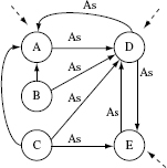
Figure 11.22 A sample ORD with five classes containing cycles between classes A, D and D, E. Dashed arrows indicate potential stubs.

11.9 How does, if any, the choice of the first node input to procedure assignMajorLevel on page 639 might affect the integration sequence output by the TD method?

11.10 In the TD method no two nodes at the same major level can be connected by an inheritance or an aggregation edge. Why?

11.11 Complete Example 11.8.

11.12 Complete Example 11.9.

11.13 Complete Example 11.10.

11.14 The TJJM algorithm ignores the types of class dependence such as aggregation, association, and inheritance. Justify this assumption.

11.15 In Example 11.11 why did we apply topological sort first to the DAG rooted at node G in Figure 11.14?

11.16 Redo Example 11.11 but assume that node B is traversed prior to traversing node F. The nodes in SCC S2 are thus traversed in the following sequence: B, H, C, A, A, E, F, and D. What differences do you observe in the outcomes of this exercise and those of Example 11.11?

11.17 At Step 2.2 in Procedure BLW, more than one edge might have the same highest weight. Show that the choice of which of these edges selected for deletion does not affect the number of specific stubs generated.

11.18 In Example 11.13 we observed that Procedure breakCycles failed to break the cycles in a subgraph. This led to a test order in which four nodes are to be tested together. Examine Step 1 in Procedure breakCycles and explain why the cycle is not broken.

11.19 Show that for a fully connected ORD having only association edges and with four or more nodes, the number of stubs generated by Procedure TD is 2.

11.20 Suggest a method for breaking cycles in clusters of classes formed when applying procedure TD. Apply your method to a fully connected ORD with six nodes and only association edges. Compare the number of stubs generated with that obtained by applying the TJJM and BLW methods.

11.21 (a) Apply the TD, TJJM, and BLW methods to generate test orders for the application shown in Figure 11.18. (b) Generate at least one test that is useful in each step of the test order, (c) For each step in the test order, indicate at least one white-box test adequacy criterion that you might use.

11.22 Suppose that components C1 and C2 contain, respectively, p₁ and p₂ paths. Assume that each of these paths is covered during unit testing. (a) Under what conditions it is not necessary to test all possible combinations of the paths when C1 and C2 are tested together? (b) What are the maximum and the minimum number of paths that might need to be tested? Provide situations where the maximum and minimum values are possible.