Chapter 4
Maxwells Equations
Maxwell’s equations are very popular and they are known as Electromagnetic Field Equations.
The main aim of this chapter is to provide sufficient background and concepts on Maxwell’s equations. They include:
- Maxwell’s equations for static and time varying fields in free space and conductive media in differential and integral form
- meaning and proof of Maxwell’s equations
- comprehensive boundary conditions in scalar and vector form
- time varying and retarded potentials
- Helmholtz theorem and Lorentz gauge condition
- points/formulae to remember, objective and multiple choice questions and exercise problems.
4.1 INTRODUCTION
Static electric field has applications in cathode ray oscilloscopes for deflecting charged particles, in ink-jet printers to increase the speed of printing and print quality, in sorting of materials in mining industry and in the development of electrostatic voltmeters.
Static magnetic field has applications in magnetic separators to separate magnetic materials from non-magnetic materials, in cyclotrons for imparting high energy to charged particles, in velocity selector and mass separators. It is also used in magnetohydrodynamic generators.
On the other hand, electromagnetic fields in their time varying form constitute electromagnetic waves. These fields/waves are useful in all communication and radar systems. In fact, the EM waves are carriers of information, mainly in free space, between the transmitter and the receiver. The electric and magnetic fields of the EM waves are related through Maxwell’s equations.
Most of the problems related to antennas can be solved with the help of Maxwell’s equations and boundary conditions. In view of this, in this chapter, Maxwell’s equations are presented in detail. Maxwell’s equations are very popular and important and hence they are also referred to as electromagnetic field equations. The fields E, H, D and B in static form are represented in Cartesian coordinates as
and
In cylindrical coordinates, they are:
and
and in spherical coordinates, they are:
and
The time varying fields E (t, x, y, z), H (t, x, y, z) constitute electromagnetic waves which have wide applications in all communications, radars and also in bio-medical engineering.
In these applications, time varying fields are of more practical value than static electric and magnetic fields.
It may be noted that electrostatic fields are usually produced by static charges. Magnetostatic fields are produced from the motion of electric charges with uniform velocity (direct current) or static magnetic charges namely magnetic dipoles.
On the other hand, time varying fields constituting EM waves are produced by time varying currents, that is, any pulsating current produces radiation fields which are nothing but time varying fields. In brief, note that:
Static charges produce electrostatic fields.
Steady currents (DC currents) produce magnetostatic fields
andstatic magnetic charges (magnetic dipoles) also produce magnetostatic fields.
Time varying currents produce EM waves or EM fields.
4.2 EQUATION OF CONTINUITY FOR TIME VARYING FIELDS
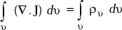
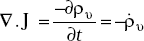
Equation of continuity in point form is
∇.J = −![]() v
v
where
|
J |
= |
conduction current density (A/m2) |
|
|
|
volume charge density (c/m3), |
|
|
|
vector differential operator |
|
|
|
|
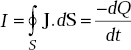
Proof Consider a closed surface enclosing a charge Q. There exists an outward flow of current given by
This is equation of continuity in integral form.
Here, I is the current flowing away through a closed surface, dS is the differential area on the surface whose direction is always outward normal to the surface. As there is outward flow of current, there will be a rate of decrease of charge given by ![]() , where Q is the enclosed charge. From the principle of conservation of charge, we have
, where Q is the enclosed charge. From the principle of conservation of charge, we have
From divergence theorem, we have
Thus, ![]()
By definition, ![]()
where ρυ = volume charge density (C/m3)
So,
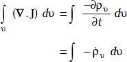
where ![]()
Two volume integrals are equal only if their integrands are equal.
Thus, ![]() Hence proved.
Hence proved.
4.3 MAXWELL’S EQUATIONS FOR TIME VARYING FIELDS
These are basically four in number.
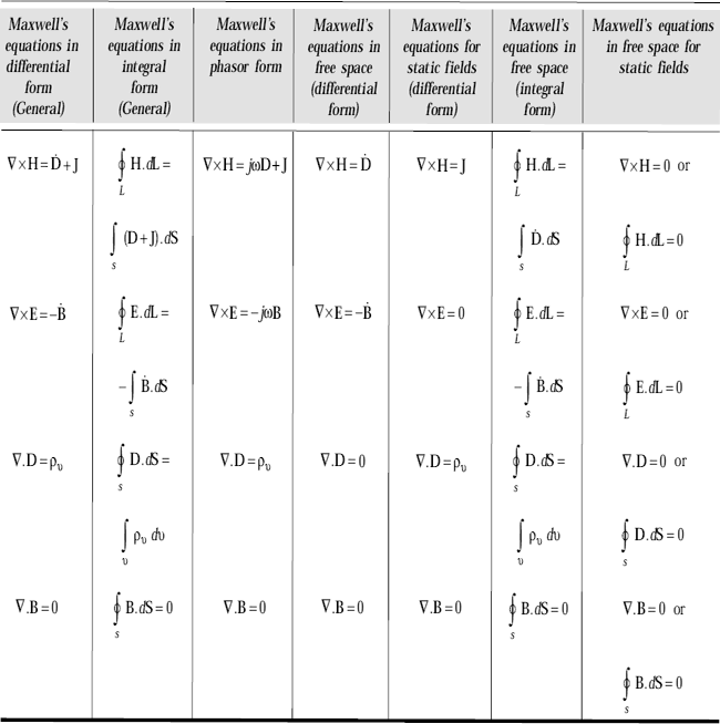
Maxwell’s equations in differential form are given by
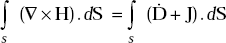
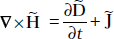
∇ × H = Ḋ + J
∇ × E = −Ḃ
∇.D = ρυ
∇.B = 0
Here
|
H |
= |
magnetic field strength (A/m) |
|
D |
= |
electric flux density, (C/m2) |
|
|
|
|
|
J |
= |
conduction current density (A/m2) |
|
E |
= |
electric field (V/m) |
|
B |
= |
magnetic flux density wb/m2 or Tesla |
|
|
|
|
Ḃ is called magnetic current density (V/m2) or Tesla/sec
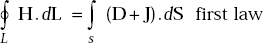
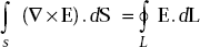
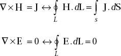
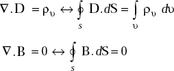
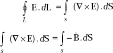
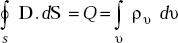
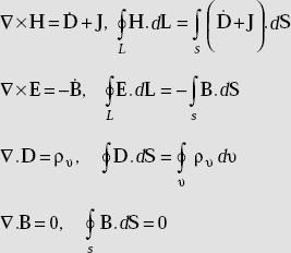
Maxwell’s equations for time varying fields in integral form are given by
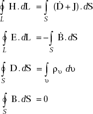
Here, dL is the differential length and dS is the differential area whose direction is always outward normal to the surface.
4.4 MEANING OF MAXWELL’S EQUATIONS
It is easy to understand the meaning of Maxwell’s equations from their integral form.
The first Maxwell’s equation states that the magnetomotive force around a closed path is equal to the sum of electric displacement and conduction currents through any surface bounded by the path.
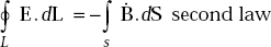
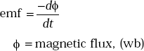
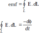
The second law states that the electromotive force around a closed path is equal to the minus of the time derivative of the magnetic flux flowing through any surface bounded by the path
orit can also be stated that the electromotive force around a closed path is equal to the inflow of magnetic current through any surface bounded by the path.
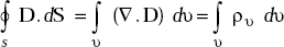
The third law states that the total electric displacement flux passing through a closed surface (Gaussian surface) is equal to the total charge inside the surface.
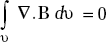
The fourth law states that the total magnetic flux passing through any closed surface is zero.
4.5 CONVERSION OF DIFFERENTIAL FORM OF MAXWELL’S EQUATION TO INTEGRAL FORM
- Consider the first Maxwell’s equation
∇ × H = Ḋ + J
Take surface integral on both sides.
Applying Stoke’s theorem to LHS, we can write
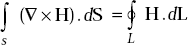
Hence
- Consider the second Maxwell’s equation
∇ × E = − Ḃ
Take surface integral on both sides.
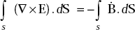
Applying Stoke’s theorem to LHS, we get
Therefore
- Consider the third Maxwell’s equation
∇.D = ρυ
Take volume integral on both sides.
Applying divergence theorem to LHS, we get
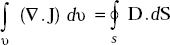
Therefore
- Consider the fourth Maxwell’s equation
∇. B = 0
Take volume integral on both sides.
Applying divergence theorem to LHS, we get
Therefore,
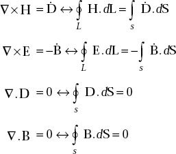
4.6 MAXWELL’S EQUATIONS FOR STATIC FIELDS
Maxwell’s equations for static fields are:
As the fields are static, all the field terms which have time derivatives are zero, that is, Ḃ = 0, Ḋ = 0.
4.7 CHARACTERISTICS OF FREE SPACE
Free space is characterised by the following parameters:
Relative permittivity, |
∈r = 1 |
|
Relative permeability, |
μr = 1 |
|
Conductivity, |
σ = 0 |
|
Conduction current density, |
J = 0 |
|
Volume charge density, |
ρυ = 0 |
|
Intrinsic impedance or characteristic impedance |
||
η = 120π or 377Ω |
||
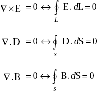
4.8 MAXWELL’S EQUATIONS FOR FREE SPACE
4.9 MAXWELL’S EQUATIONS FOR STATIC FIELDS IN FREE SPACE
4.10 PROOF OF MAXWELL’S EQUATIONS
- From Ampere’s circuital law, we have
∇ × H =J
Take dot product on both sides
∇ . ∇ × H = ∇ . JAs the divergence of curl of a vector is zero,
RHS = ∇. J = 0But the equation of continuity in point form is
This means that if ∇ × H = J is true, it is resulting in ∇. J = 0.
As the equation of continuity is more fundamental, Ampere’s circuital law should be modified. Hence we can write
∇ × H = J + FTake dot product on both sides
∇ . ∇ × H = ∇ . J + ∇.Fthat is,
∇ . ∇ × H = 0 = ∇ . J + ∇.FSubstituting the value of ∇ .J from the equation of continuity in the above expression, we get
∇.F + (− υ) = 0
or,
∇.F =υThe point form of Gauss’s law is
∇ . D = ρυor,
∇ . Ḋ =υFrom the above expressions, we get
∇ . F = ∇ . ḊThe divergence of two vectors are equal only if the vectors are identical,
that is, F = Ḋ
So, ∇ × H = Ḋ + J Hence proved.
- According to Faraday’s law,
and by definition,
But
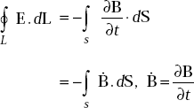
Applying Stoke’s theorem to LHS, we get
Two surface integrals are equal only if their integrands are equal,
that is, ∇ × E = − Ḃ Hence proved.
- From Gauss’s law in electric field, we have
Applying divergence theorem to LHS, we get
Two volume integrals are equal if their integrands are equal,
that is ∇ . D = ρυ
Hence
- We have Gauss’s law for magnetic fields as

RHS is zero as there are no isolated magnetic charges and the magnetic flux lines are closed loops.
Applying divergence theorem to LHS, we get
or, ∇.B = 0 Hence proved.
4.11 SINUSOIDAL TIME VARYING FIELD
In practice, electric and magnetic fields vary sinusoidally. It is well-known that any periodic variation can be described in terms of sinusoidal variations with fundamental and harmonic frequencies.
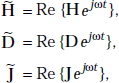
The fields can be represented by
or,
where ω = 2π f, f = frequency variation of the field, Em is the maximum field strength.
It means that a sinusoidal time factor is attached to the field. It is also possible to represent the fields using phasor notation. The time varying field Ẽ (r, t) is related to phasor field E (r) as
or,
It may be noted that cosinusoidal variation is also considered to be sinusoidal in usage.
4.12 MAXWELL’S EQUATIONS IN PHASOR FORM
- Consider the first Maxwell’s equation
If
it becomes,
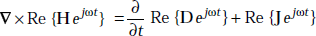
or, Re {∇ × H − jωD − J) ejωt} = 0
or, ∇ × H = jωD + J
This is the first Maxwell’s equation in phasor form.
- Consider the second Maxwell’s equation

If Ẽ = Re {E ejωt}
and
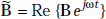
the second Maxwell’s equation becomes,
or, Re [(∇ × E + jωB) ejωt] = 0
or, ∇ × E = − jωB
This is the second Maxwell’s equation in phasor form.
- Similarly, consider the third Maxwell’s equation,

that is, ∇.Re (D ejωt) = ρυ
or, ∇.D = ρυ
- Consider the fourth Maxwell’s equation

that is, ∇.Re (B ejωt) = 0
or, ∇.B = 0
In summary, Maxwell’s equations in phasor form are:
∇ × H = jωD + J
∇ × E = −jωB
∇.D = ρυ
∇.B = 0
4.13 INFLUENCE OF MEDIUM ON THE FIELDS
When the sources of electric and magnetic fields exist in a medium, the medium has influence on the characteristics of the fields. The constitutive relations, namely,
describe the characteristics.
Here ∈ = permittivity (F/m), μ = permeability (H/m) and σ = conductivity (mho/m) of the medium.
4.14 TYPES OF MEDIA
Medium can be divided into five types:
- Homogeneous medium
- Non-homogeneous medium
- Isotropic medium
- Anistropic medium
- Source-free regions
- Homogeneous medium It is a medium for which ∈, μ and σ are constant throughout the medium.
Example Free space.
- Non-homogeneous medium It is a medium for which ∈, μ and σ are not constants and are different from point to point in the medium.
Example Human body.
- Isotropic medium It is a medium for which ∈ is a scalar constant.
Example Free space.
- Anistropic medium It is a medium for which ∈ is not a scalar constant.
Example Human body.
- Source–free region It is a medium in which there are no field sources.
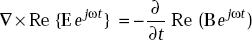
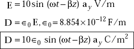
Problem 4.1 Given E = 10sin (ωt –βz) ay V/m in free space, determine D, B, H.
Solution
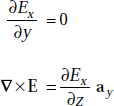
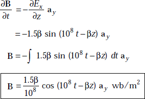
Second Maxwell’s equation is
that is,
or,
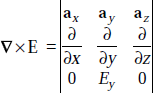
As
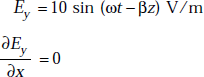
Now ∇ × E becomes
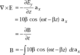
or,
and

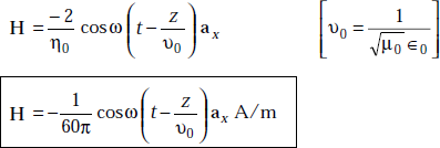
Problem 4.2 If the electric field strength, E of an electromagnetic wave in free space is given by 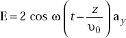 V/m find the magnetic field, H.
Solution We have
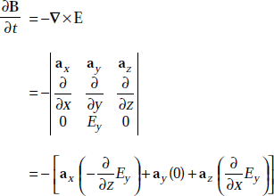
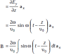
or,
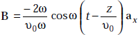
or,
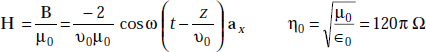
Thus,
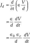
Problem 4.3 The parallel plates in a capacitor have an area of 4 x 10⁻⁴ m2 and are separated by 0.4 cm. A voltage of 10 sin 103 t volts is applied to the capacitor. Find the displacement current when the dielectric material between the plates has a relative permittivity of 4.
Solution We have
or,
The displacement current density, Jd is
But
where d = plate separation = 0.4 cm = 0.004 m.
So,
The displacement current, Id is
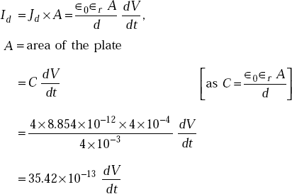
But V = 10 sin 103 t volt
So,
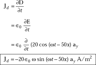
Problem 4.4 In free space, the magnetic field of an EM wave is given by H = 0.4ω∈0 cos (ωt – 50x) az A/m. Find the electric field, E and displacement current density, Ḋ.
Solution H = 0.4ω∈0 cos (ωt – 50x) az A/m
We have ∇ × H = Ḋ + J
But J = 0 for free space.
So,
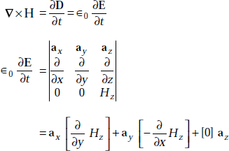
But
[H is not a function of y]
So,
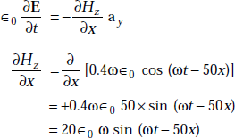
that is,
or,
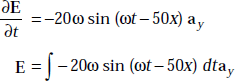
The displacement current density, Jd
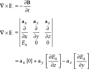
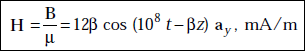
Problem 4.5 If there is a magnetic field represented by
in a medium where ρυ = 0, σ = 0 and J = 0, find the electric field. Assume ∈r = 1, μr = 1.
Solution We have ∇ × H = Ḋ + J
But J = 0
as D = ∈0E, B = μ0 H
We can write ![]()
or, ![]()
or,
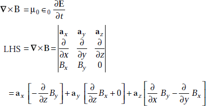
As Bx and By are independent of y and z,
But
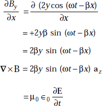
or,
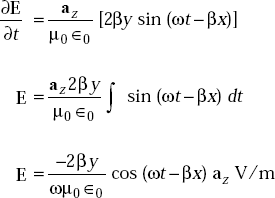
Problem 4.6 An electric field in a medium which is source-free is given by E = 1.5 cos (108t – βz)ax V/m, where Em is the amplitude of E, ω is the angular frequency and β is the phase constant. Obtain B, H, D. Assume ∈r = 1, μr = 1, σ = 0.
Solution We have
As Ex is not a function of y,
or,
As B = μ H, μ = μ0 = 4 π × 10−7 H/m
But D = ∈ E = ∈0E, ∈0 = 8.854 × 10⁻¹² F/m
So,
Problem 4.7 Verify whether the following fields
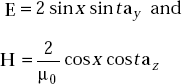
satisfy Maxwell’s equations in free space.
Solution ∇ × H = Ḋ
[as J = 0]
that is,
or, ![]() sin x cost = 2∈0 sin x cost
sin x cost = 2∈0 sin x cost
or, μ0∈0 = 1
which cannot be satisfied. Therefore, the given fields do not satisfy Maxwell’s equations.
Problem 4.8 In a medium of conduction current density given by
find the volume charge density.
Solution J = 3.0sin (ωt – 10z)ay + cos (ωt- 10z)az
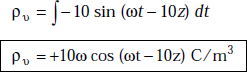
By the equation of continuity, we have
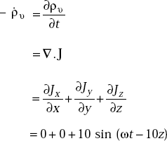
that is, ![]() υ = −10 sin (ωt − 10z)
υ = −10 sin (ωt − 10z)
or,
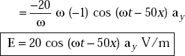
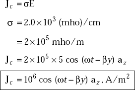
Problem 4.9 If the electric field strength of a radio broadcast signal at a TV receiver is given by
determine the displacement current density. If the same field exists in a medium whose conductivity is given by 2.0 × 10³ (mho)/cm, find the conduction current density.
Solution E at a TV receiver in free space
Electric flux density,
The displacement current density
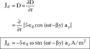
The conduction current density,
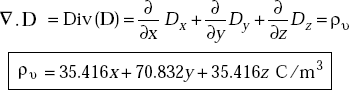
Problem 4.10 Find the electric flux density and volume charge density if the electric field,
in a medium whose ∈r = 2.
Solution
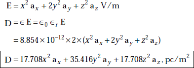
From Maxwell’s equation, we have
4.15 SUMMARY OF MAXWELL’S EQUATIONS FOR DIFFERENT CASES
4.16 CONDITIONS AT A BOUNDARY SURFACE
Relations between the main fields E, D, H, B are expressed in terms of Maxwell’s equations. These are valid at any point in a continuous medium.
As Maxwell’s equations contain space derivatives, they cannot give information at points of discontinuity in the medium. However, Maxwell’s equations in integral form can be used to get the information at the boundary surface between different media.
The electromagnetic fields that are solved using Maxwell’s equations must satisfy boundary conditions at the interface between different media.
The boundary conditions on electric and magnetic fields at any surface of discontinuity are given by:
- The tangential component of electric field, E is continuous across any discontinuity, that is,
Etan1 = Etan2
Subscript tan 1 is the tangential component of the field at the boundary in medium 1. Subscript tan 2 represents it in medium 2.
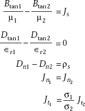
- The tangential component of magnetic field, H is continuous across any surface except at the surface of a perfect conductor. At the surface of a perfect conductor, the tangential component of H is discontinuous by quantity equal to the surface current density (A/m).
Htan1 − Htan2 = Js
- The normal component of B is continuous across any discontinuity.
Bn1 = Bn2
- The normal component of D is continuous except at a surface which has surface charge density. At the surface where surface charge density exists, the normal component of D is discontinuous by a quantity equal to the surface charge density.
Dn1 − Dn2 = ρs
Subscript n1 represents normal component of the field in medium 1 and n2 represents it in medium 2.
4.17 PROOF OF BOUNDARY CONDITIONS ON E, D, H AND B
To Prove Etan1 = Etan2
Consider the rectangular loop on the boundary of two media (Fig. 4.1).
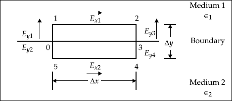
Fig. 4.1 Rectangular loop on boundary
It is well-known that electric field is conservative and hence the line integral of E . dL is zero around a closed path.
So,
From the figure shown above, LHS is written as
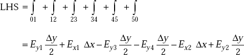
As Δy → 0, we get
or, Ex1 = Ex2
It is obvious that Ex1 and Ex2 are the tangential components of E in medium 1 and 2 respectively.
So, Etan1 = Etan2
Now consider a cylinder across the media 1 and 2 (Fig. 4.2).
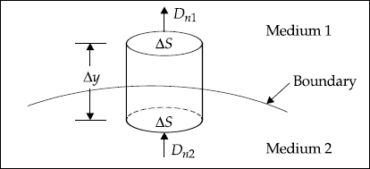
Fig. 4.2 Cylinder across boundary
According to Gauss’s law,
Applying this to the cylindrical surface on the boundary spreading over medium 1 and medium 2, we get, as Δy → 0
or,
To Prove Htan1 – Htan2 = Js
Consider the rectangular loop on the boundary of two media (Fig. 4.3).
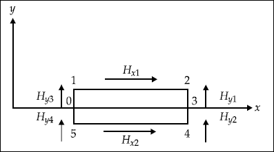
Fig. 4.3 A rectangular loop across a boundary
From Ampere’s circuit law, we have
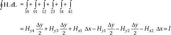
As Δy → 0, we get
or,
Here, Hx1 and Hx2 are nothing but tangential components in medium 1 and 2 respectively.
To prove Bn1 = Bn2
Now consider a cylinder shown in Fig. 4.4.
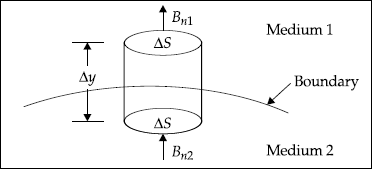
Fig. 4.4 A differential cylinder across the boundary
Gauss’s law for magnetic fields is
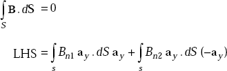
Applying LHS to the cylindrical surfaces shown, we get, for Δy → 0
Given the fields in one medium, it is usually required to determine fields in a second medium. This requires the knowledge of both tangential and normal components for each field. The above boundary conditions yield either tangential or normal component. The second unknown component is determined from the constitutive relations between E and D, H and B.
We have Etan 1 = Etan 2
But D = ∈ E
We have Dn1 − Dn2 = ρs
We have Bn1 = Bn2
But
B = μH
μ1 Hn1 = μ2 Hn2
We have Htan 1 − Htan 2 = Js
4.18 COMPLETE BOUNDARY CONDITIONS IN SCALAR FORM
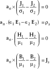
Etan 1 − Etan 2 = 0
∈1 En1 − ∈2 En2 = ρs
Htan 1 − Htan 2 = Js
μr1 Hn1 − μr2 Hn2 = 0
Bn1 − Bn2 = 0
4.19 BOUNDARY CONDITIONS IN VECTOR FORM
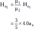
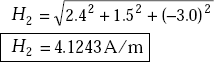
Problem 4.11 x < 0 defines region 1 and x > 0 defines region 2. Region 1 is characterised by μr1 = 3.0 and region 2 is characterised by μr2 = 5.0. If the magnetic field in region 1 is given by H1 = 4.0ax + 1.5ay – 3.0az, A/m, find H2 and H2.
Solution H1 = 4.0ax + 1.5ay – 3.0az, A/m
For the regions given,
and ![]()
As
and
or, ![]()
and, ![]()
The magnitude of H2 is
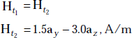
Problem 4.12 In a three-dimensional space, divided into region 1 (x < 0) and region 2 (x > 0), σ1 = σ2 = 0. E1 = 1ax + 2ay + 3az. Find E2 and D2.∈r1 = 1 and ∈r2
Solution |
Et1 = 2ay + 3az, V/m |
|
En1 = ax , ∈r1 = 1 |
|
Dt1 = ∈0 (2ay + 3az ), C/m2 |
As |
Et1 = Et2 |
|
Et2 = 2ay + 3az , V/m |
As |
Dn1 = Dn2 |
|
∈1 En1 = ∈2En2 |
or,
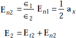
or, ![]()
D2 = ∈2E2
= 2 ∈0 (0.5ax + 2ay + 3az)
or, ![]()
4.20 TIME VARYING POTENTIALS
It is always useful to relate electric and magnetic fields in terms of their sources. However, it is often more convenient to relate potentials in terms of sources and then the fields in terms of potentials.
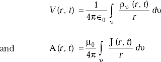
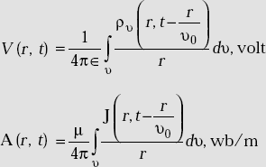
In the first method potentials already developed for static fields are generalised to obtain time varying fields. Scalar electrostatic potential is given by
and vector magnetic potential is
But the time varying potentials are expressed in the form of
These time varying potentials are due to time varying charge and current distributions.
The above expressions do not take care of propagation delay. To obtain far-field expressions, this delay time must be taken into account.
4.21 RETARDED POTENTIALS
These are defined as the potentials in which a time delay or retarded time is taken into account. They are expressed as:
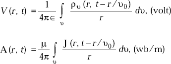
where retarded time or delay time is
td = (t − r/υ0)
υ0 = velocity of propagation of the EM wave
From the above approach, there is no change in the expressions for E and H, that is,
E = − ∇V
and ![]()
4.22 MAXWELL’S EQUATIONS APPROACH TO RELATE POTENTIALS, FIELDS AND THEIR SOURCES
By definition, vector magnetic potential, A is related to magnetic flux density as
But the second Maxwell’s equation is
From the above two expressions, we have
or, ∇ × E + ∇ × Ȧ = 0
or, ∇ × (E + Ȧ = 0
This is true only if (E + Ȧ) is the gradient of a scalar. Therefore, setting (E + Ȧ) = – ∇V, we get E as
Note that E is not equal to (−∇V) for time varying fields but it is given by the above expression.
So, E = − ∇V is valid only for static fields
Now consider
Take curl on both sides,
or,
But ∇ × H = Ḋ + J = ∈0 Ė + J
From the above expressions, we get
∈0 Ė + J =− ∈0 ∇ ![]() − ∈0 Ä + J
− ∈0 Ä + J
![]() ∇ × ∇ × A = −∈0 ∇V − ∈0 Ä + J
∇ × ∇ × A = −∈0 ∇V − ∈0 Ä + J
But vector identity gives
that is, ∇∇.A − ∇2 A = μ0 ∈0 ∇![]() − μ0 ∈0 Ä + μ0 J
− μ0 ∈0 Ä + μ0 J
The third Maxwell’s equation is
This becomes ∇.E = − ∇.∇V − ∇.Ȧ = ρυ/∈0
or, ∇2V + ∇Ȧ = −ρυ/∈0
and ∇2 A − μ0 ∈0 Ä = −μ0 J + μ0 ∈0 ∇![]() + ∇∇.A
+ ∇∇.A
Each of the equations contain both the potentials and one of the sources. It is difficult to solve such type of equations. We should be able to get equations containing one potential and its own source to solve them easily. Helmholtz theorem helps to do this.
4.23 HELMHOLTZ THEOREM
It states that any vector field like A due to a finite source is uniquely specified if and only if its curl and the divergence are specified.
To specify A, we know its curl, that is,
But the ∇.A is specified as
and ∇2 V − μ0 ∈0 ![]() = −ρυ/∈0
= −ρυ/∈0
These are the expressions between time varying potentials and their sources.
The corresponding expressions for static fields are:
4.24 LORENTZ GAUGE CONDITION
It is given by
Potential functions for sinusoidal fields are given by
∇2 A + ω2 μ0 ∈0 A = −μ0 J
∇2 V + ω2 μ0 ∈0 V = −ρυ/∈0
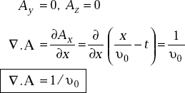
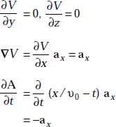
Problem 4.13 If the retarded scalar electric potential, V = x – υ0t and vector magnetic potential, 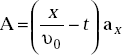 where υ0 is the velocity of propagation,
- find ∇. A
- find B, H, E, and D
- show that

Solution (a)
But
(b) We have B = ∇ × A
Here
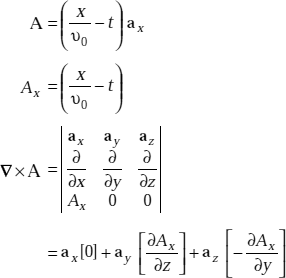
As ![]() and Ax is not function of z,
and Ax is not function of z,
Therefore, ∇ × A = 0
and ![]()
As
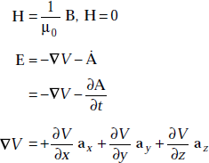
Here
or, E = − ∇V − Ȧ
and
(c) ![]()
But ![]()
or,
 Hence proved.
POINTS/FORMULAE TO REMEMBER
- Maxwell’s equations are electromagnetic field equations.
- Maxwell’s equations give relations between different fields and sources.
- Equation of continuity is ∇.J =

- Most general Maxwell’s equations are
- For static fields, Ḃ = 0, Ḋ = 0.
- In good dielectrics, J = 0.
- In good conductors, Ḋ = 0.
- For free space, ρυ = 0, J = 0, σ = 0.
- For conducting media, ρυ = 0
 is known as the magnetic current density.
- Magnetic current density has the unit of volt/m2.
- Maxwell’s equations in phasor form are:
∇ × H = jωD + J∇ × E = −jωB∇.D = ρυ∇.B = 0
- The constitutive relations are:
D = ∈ EB = μ HJ = σ E
- For a homogeneous medium, ∈, μ, σ are constants throughout the medium.
- For isotropic medium, ∈ is a scalar constant.
- Retarded potentials are:
- For time varying fields, E = − ∇V − Ȧ
- According to Helmholtz theorem, if the curl and divergence of a vector are specified, it exhibits unique meaning.
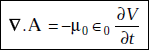
- Lorentz gauge condition is ∇.A = −μ0 ∈0

OBJECTIVE QUESTIONS
1. E = – ∇ V is valid for all types of fields. |
(Yes/No) |
2. |
(Yes/No) |
3. Theta polarisation is called linear polarisation. |
(Yes/No) |
4. B and D can be related. |
(Yes/No) |
5. The characteristic impedance of a medium is |
|
6. |
(Yes/No) |
7. ∇.E =− Ḃ |
(Yes/No) |
8. ∇.J = |
(Yes/No) |
9. In free space, ∇. D = 0. |
(Yes/No) |
10. In free space, ∇ × H = J. |
(Yes/No) |
11. For static fields, ∇ × H = D. |
(Yes/No) |
12. The unit of D is wb/m2. |
(Yes/No) |
13. The unit of Ḋ is A/m2. |
(Yes/No) |
14. The unit of J is A/m. |
(Yes/No) |
15. E and D have the same direction. |
(Yes/No) |
16. B and H have the same direction. |
(Yes/No) |
17. Ampere’s circuit law and Maxwell’s first equation are the same. |
(Yes/No) |
18. Bn1 is always equal to Bn2. |
(Yes/No) |
19. Dn1 is always equal to Dn2. |
(Yes/No) |
20. Etan 1 is always equal to Etan2. |
(Yes/No) |
(Yes/No) |
|
22. Surface current density in dielectrics is zero. |
(Yes/No) |
23. ρυ = 0 for free space. |
(Yes/No) |
24. In dielectrics, displacement current density is greater than conduction current density. |
(Yes/No) |
25. In conductors, Jc > Jd. |
(Yes/No) |
26. ∇. B = 0 because there exists no isolated magnetic poles. |
(Yes/No) |
27. The unit of vector magnetic potential is _____. |
|
28. The unit of magnetic current density is _____. |
|
29. If E = cos (6 × 10⁷ t −β z) ax, β is _____. |
|
30. For time varying fields, E = _____. |
|
Answers
1. Yes |
2. Yes |
3. Yes |
4. Yes |
5. No |
6. No |
7. No |
8. No |
9. Yes |
10. No |
11. No |
12. No |
13. Yes |
14. No |
15. Yes |
16. Yes |
17. No |
18. Yes |
19. No |
20. Yes |
21. No |
22. Yes |
23. Yes |
24. Yes |
25. Yes |
26. Yes |
27. Wb/m |
28. V/m |
29. 0.2 rad/m |
30. − ∇V − Ȧ |
|
|
MULTIPLE CHOICE QUESTIONS
- The first Maxwell’s equation in free space
- ∇ × H = Ḋ + J
- ∇ × H = Ḋ
- ∇ × H = 0
- ∇ × H = J
- Absolute permeability of free space is
- 4π × 10-7 A/m
- 4π × 10-7 H/m
- 4π × 10-7 F/m
- 4π × 10-7 H/m2
- For static magnetic field,
- ∇ × B = ρ
- ∇ × B = μJ
- ∇ × B = μ0J
- ∇ × B = 0
- The electric field in free space


- ∈0 D

- Displacement current density is
- D
- J
- ∂D/∂t
- ∂J/∂t
- The time varying electric field is
- E = − ∇V
- E = − ∇V − Ȧ
- E = − ∇V − B
- E = − ∇V − D
- A field can exist if it satisfies
- Gauss’s law
- Faraday’s law
- Coulomb’s law
- All Maxwell’s equations
- If σ = 2.0 mho/m, E = 10.0 V/m, the conduction current density is
- 5.0 A/m2
- 20.0 A/m2
- 40.0 A/m2
- 20 A
- Maxwell’s equations give the relations between
- different fields
- different sources
- different boundary conditions
- none of these
- The boundary condition on E is
- an × (E1 − E2) = 0
- an.(E1 − E2) = 0
- E1 = E2
- none of these
- The boundary conditions on H is
- an × (H1 − H2) = Js
- an .(H1 − H2) = 0
- an × (H1 − H2) = Js
- an .(H1 − H2) = 0
- If E = 2 V/m, of a wave in free space, (H) is

- 60 πA/m
- 120 πA/m
- 240 πA/m
- cosine of the angle between the two vectors is
- sum of the products of the directions of the two vectors
- difference of the products of the directions of the two vectors
- product of the products of the directions of the two vectors
- none of these
- The electric field intensity, E at a point (1, 2, 2) due to (1/9) nc located at (0, 0, 0) is
- 33 V/m
- 0.333 V/m
- 0.33 V/m
- zero
- If E is a vector, then ∇ . ∇ × E is
- 0
- 1
- does not exist
- none of these
- The Maxwell’s equation, ∇. B = 0 is due to
- B = μ H

- non-existence of a mono pole
- none of these
- For free space,
- σ = ∞
- σ =0
- J ≠ 0
- none of these
- The electric field for time varying potentials
- E = − ∇V
- E = − ∇V − A
- E = ∇V
- E = − ∇V + A
- The intrinsic impedence of the medium whose σ = 0, ∈r = 9, μr = 1 is
- 40 πΩ
- 9 Ω
- 120 πΩ
- 60 πΩ
- For time varying EM fields
- ∇ × H = J
- ∇ × H = Ḋ + J
- ∇ × E = 0
- none of these
- The wavelength of a wave with a propagation constant = 0.1π + j 0.2π is
- 10 m
- 20 m
- 30 m
- 25 m
- The electric field just above a conductor is always
- normal to the surface
- tangential to source
- zero
- ∞
- The normal components of D are
- continuous across a dielectric boundary
- discontinuous across a dielectric boundary
- zero
- ∞
- If Jc = 1 mA/m2 in a medium whose conductivity is σ = 10 Mho/m, E is
- 0.1 V/m
- 10μ V/m
- 1.0μ V/m
- 10 V/m.
- If Jd = 2 mA/m2 in a medium whose ∈r = 2, σ= 4.95 Mho/m at a frequency of 1 GHz, Jc is
- 8.9 mA/m2
- 89 mA/m2
- 0.89 mA/m2
- 89 A/m2
Answers
1. (b) |
2. (b) |
3. (b) |
4. (a) |
5. (c) |
6. (b) |
7. (d) |
8. (b) |
9. (a) |
10. (a) |
11. (b) |
12. (a) |
13. (a) |
14. (c) |
15. (a) |
16. (c) |
17. (b) |
18. (a) |
19. (a) |
20. (b) |
21. (a) |
22. (a) |
23. (a) |
24. (a) |
25. (b) |
|
|
|
EXERCISE PROBLEMS
- If A is the vector magnetic potential, prove
- If E = 2.0 sinkx cosωtax in free space, find the volume charge density.
- If E = 10 cos (ωt – kz)ax V/m, find D, H, B in free space.
- If the electric field strength of an EM wave in free space has an amplitude of 5.0 V/m, find the magnetic field strength.
- When the amplitude of a magnetic field in free space is 10 mA/m, find the magnitude of the electric field.
- The electric field of an EM wave is
 Find H.
 - If Ẽ = 2 cos (108t – 20x + 40°)az, what is the phasor form of E?