Chapter 7
Transmission Lines
Transmission lines are nothing but guided conducting structures which are used in power distribution at low frequencies, in communications and computer networks at higher frequencies.
The main aim of this chapter is to provide the overall concepts of Transmission Line theory. They include:
- transmission lines and applications
- equivalent circuits
- primary and secondary constants
- lossless and distortionless lines
- loading of lines and RF lines
- reflection coefficient and VSWR
- stubs and smith charts
- solved problems, points/formulae to remember, objective and multiple choice questions and exercise problems.
7.1 TRANSMISSION LINES
A transmission line is a means of transfer of information from one point to another. Usually it consists of two conductors. It is used to connect a source to a load. The source may be a transmitter and the load may be a receiver.
7.2 TYPES OF TRANSMISSION LINES
The various types of transmission lines are
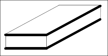
- Two-wire parallel lines
- Coaxial lines
- Twisted wires
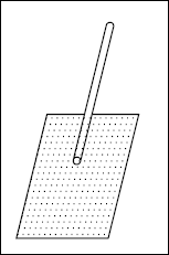
- Parallel plates or planar lines
- Wire above conducting line
- Microstrip lines
- Optical fibres
Typical configurations of the above are shown in Fig. 7.1.
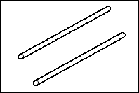
(a) Two-wire parallel line
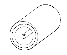
(b) Coaxial line
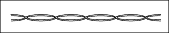
(c) Twisted pair of lines
(d) Planar line
(e) Wire above conducting plane
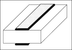
(f) Microstrip line
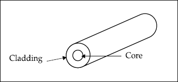
(g) A typical step-index optical fibre
Fig. 7.1 Types of transmission lines
7.3 APPLICATIONS OF TRANSMISSION LINES
Applications of transmission lines are:
- They are used to transfer energy from one circuit to another.
- They can be used as circuit elements like inductors, capacitors and so on.
- They can be used as impedance matching devices.
- They can be used as stubs.
- They can be used as measuring devices.
- Coaxial cables are frequently used in laboratories and to connect televisions to TV antennas.
- Microstrips are used in integrated circuits in which metallic strips connecting electronic elements are deposited on dielectric substrates.
- Twisted pairs and coaxial cables are used in computer networks such as Ethernet and Internet.
- Pair of parallel lines are used in telephony and power transmission.
- Planar lines are used to connect transmitters and antennas.
- Optical fibres are used to transmit information over long and short distances with negligible attenuation.
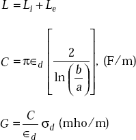
7.4 EQUIVALENT CIRCUIT OF A PAIR OF TRANSMISSION LINES
The equivalent circuit of a transmission line is a distributed network. This consists of cascaded sections and each section consists of a series Resistance R, series Induction L, shunt Capacitance C, and shunt conductance G. One section of the equivalent circuit is shown in Fig. 7.2. Here R is expressed in ohm/unit length, L in Henry/unit length, C in Farad/unit length and G in Mho per unit length.
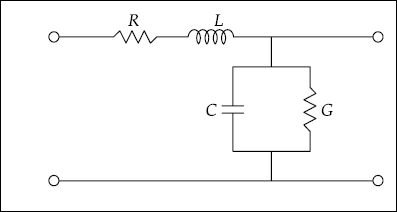
Fig. 7.2 Equivalent circuit of a two-conductor transmission line
Electric and Magnetic Fields in Parallel Plate and Coaxial Lines
In parallel plate transmission, if z is the direction of propagation, the electric and magnetic field distributions are shown in Fig. 7.3.
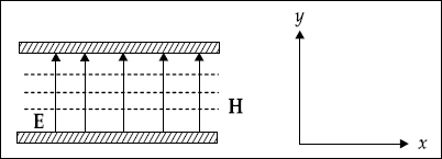
Fig. 7.3 E and H in a parallel plate transmission line
The E and H fields in a coaxial line are shown in Fig. 7.4.
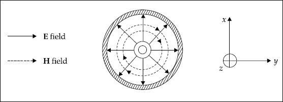
Fig. 7.4 E and H fields in a coaxial line
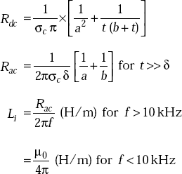
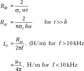
7.5 PRIMARY CONSTANTS
The R (Ω /Km), L (H/Km), C (F/Km) and G (mho/Km) are known as primary constants.
Salient aspects of primary constants:
- R is defined as loop resistance per unit length of line.
- L is defined as loop inductance per unit line length.
- C is defined as shunt capacitance between two wires per unit length.
- G is defined as the conductance per unit length due to the dielectric medium separating the conductors. It may be noted that

- R, L, C, G are distributed along the length of the line.
- For each line, the conductors are characterised by σc and μc = μ0, ∊c = ∊0, and the dielectric medium, which is basically homogeneous, separating the conductor is characterised by σd, μd, ∊d
- R, L, C and G depend on the geometry of transmission line, characteristics of the dielectric material and in some cases on the frequency.
The relations are presented for quick reference.
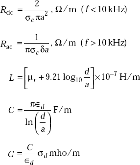
For parallel wires
where |
σc |
= |
conductivity of conductors |
|
a |
= |
radius of wire |
|
|
|
|
|
d |
= |
spacing between wires |
|
∊d |
= |
dielectric constant of the dielectric material |
|
μr |
= |
relative permeability of the conductor material |
|
|
= |
1 for non-magnetic material |
Internal inductance (Li) is due to internal flux linkages in the conductors.
It is
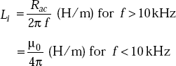
External inductance (Le) is due to flux linkages with the flux external to the wire.
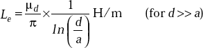
For coaxial cable
where |
a |
= |
inner radius |
|
b |
= |
outer radius |
|
t |
= |
outer thickness |
For parallel plates
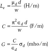
where |
w |
= |
width |
|
d |
= |
separation |
7.6 TRANSMISSION LINE EQUATIONS
Consider Fig. 7.5 in which a line of length l, voltage and current at source end, Vs and Is are shown. The voltage, VL and current IL at the load end are also shown.
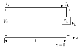
Fig. 7.5 A transmission line with load, ZL
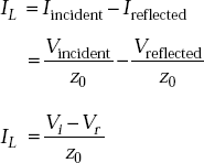
Let V and I be the voltage and current on the line at any arbitrary location. Assume Vf and If are for the forward wave and Vr and Ir are for the reflected wave. Then, we can write
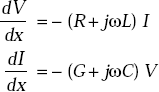
Differentiating and combining, we get
where |
γ2 |
= |
(R + jωL) (G + jωC) |
or, |
γ |
= |
|
|
|
= |
propagation constant |
And the series impedance
The shunt admittance
The solutions of Equations (7.1) and (7.2) are either in exponential form or in hyperbolic function form. In the first form,
These represent the sum of the forward and reflected waves.
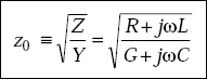
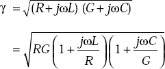
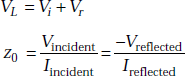
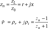
The characteristic impedance,
z0 is related to R, L, C and G and is given by
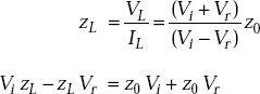
If the line is terminated in a load impedance of zL, then
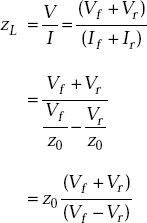
or, zL Vf − zL Vr = z0 Vf + z0 Vr
Dividing both sides by Vf, we get
or,
or,
The reflection coefficient,
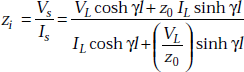
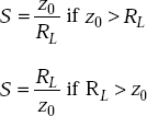
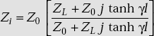
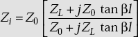
7.7 INPUT IMPEDANCE OF A TRANSMISSION LINE
Input impedance zi is defined as the ratio of voltage and current at the sending end.
In hyperbolic function form, the solutions of Equations (7.1) and (7.2) are given by
The constants, A1, A2, B1 and B2 are found using the boundary conditions, that is,
Then
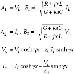
zL is chosen at x = 0 and if l = −x, we have
Here, l is measured from the load end. From Equations (7.3) and (7.4), we have
If the line is short circuited at the receiving end, zL = 0 and VL = 0. Then the input impedance is
Now if zL = ∞, IL = 0, then the input impedance is
or, ![]()
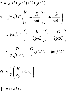
7.8 SECONDARY CONSTANTS
The secondary constants are
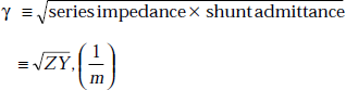
Propagation constant, γ and
Characteristic impedance, z0
Propagation constant
Definition 1
Definition 2 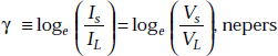
Definition 3 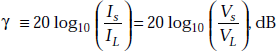
Definition 4 γ ≡ α + jβ
where |
α |
= |
attenuation constant, dB/m |
|
β |
= |
phase constant, rad/m |
It may be noted that
Consider
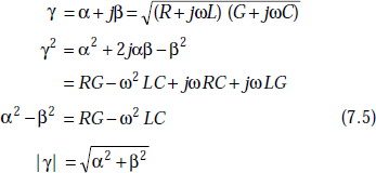
From Equations (7.5) and (7.6), we have
or,
From Equations (7.6) and (7.7), we get
or,
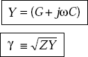
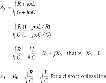
Characteristic impedance, z0
Definition 1 The characteristic impedance, z0 of a line is defined as the ratio of the forward voltage wave to the forward current wave at any point on the line,
that is,
Definition 2 z0 is also defined as the ratio of the square root of series impedance to the square root of shunt admittance, or,
Definition 3 z0 is defined as the minus of the ratio of the reflected voltage wave to the reflected current wave at any point on the line, or,
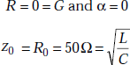
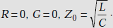
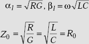
7.9 LOSSLESS TRANSMISSION LINES
A transmission line is said to be lossless if the conductors of the line are perfect, or, σc = ∞ and the dielectric medium between the lines is lossless, or, σd = 0. Also, a line is said to be lossless, if
For lossless line,
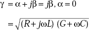
As R = 0, G = 0
or,
As R = 0 = G
The velocity of propagation in lossless line
7.10 DISTORTIONLESS LINE
A transmission line is said to be distortionless when the attenuation constant, α is frequency-independent and the phase constant, β is linearly dependent on the frequency or when
Consider
If
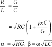
Consider
The velocity of propagation for distortionless line is
The overall transmission line characteristics are shown in Table 7.1.
Table 7.1 Propagation Parameters for Different Types of Lines
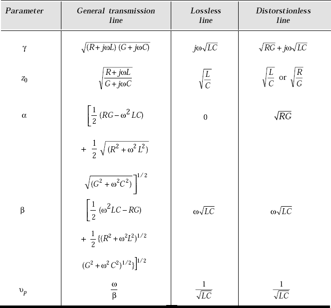
7.11 PHASE AND GROUP VELOCITIES
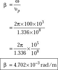
Energy is propagated along a transmission line in the form of Transverse Electromagnetic wave (TEM wave). The phase velocity, υp for TEM wave is
For a transmission line, μr = 1, but ∊r may be different. Then
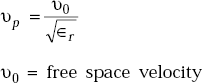
For a lossless and distortionless transmission line,
Individual waves propagate with the same phase velocity if β is proportional to ω. If β is not proportional to ω and if the wave components travel with different velocities, the envelope of the wave travels with a velocity, known as group velocity, υg, that is,
This is also the velocity at which energy is propagated along the line.
7.12 LOADING OF LINES
Introduction of inductance in series with the line is called loading and such lines are called loaded lines.
Effect of loading
This is shown in Fig. 7.6.
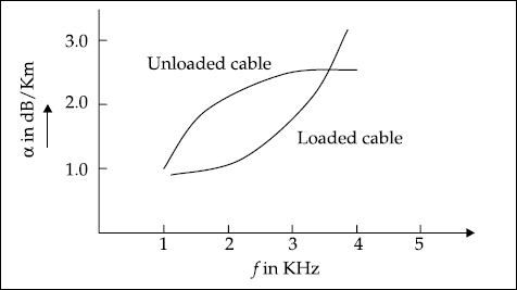
Fig. 7.6 Effect of loading on the cable
Types of loading
- Continuous loading Here loading is done by winding a type of iron around the conductor. This increases inductance but it is expensive.
- Patch loading This type of loading uses sections of continuously loaded cable separated by sections of unloaded cable. Hence cost is reduced.
- Lumped loading Here, loading is introduced at uniform intervals. It may be noted that hysteresis and eddy current losses are introduced by loading and hence design should be optimal.
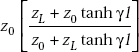
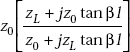
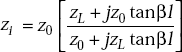
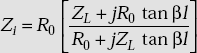
7.13 INPUT IMPEDANCE OF LOSSLESS TRANSMISSION LINE
For lossless line,
and as tanh jβl = j tan βl and z0 = R0 , zi becomes
 (for a lossless line)
For shorted line, zL = 0
For open circuited line, zL = ∞
and ![]()
Input impedances of a transmission line for different cases are given in Table 7.2.
Table 7.2 Input Impedance for Different Loads
| Type of line | Input impedance, zi |
|---|---|
Lossy line |
 |
Lossless line |
 |
Lossy line with shorted load (zL = 0) |
z0 tanh β l |
Lossy line with open circuited load (zL = ∞) |
z0 coth βl |
Lossy line with matched load (zL = z0) |
z0 |
Lossless line with shorted load |
j z0 tan βl |
Lossless line with open circuited load |
− j z0 cot βl |
Lossless line with matched load |
z0 |
The variation of input impedance of lossless line when shorted and open circuited are shown in Fig. 7.7.
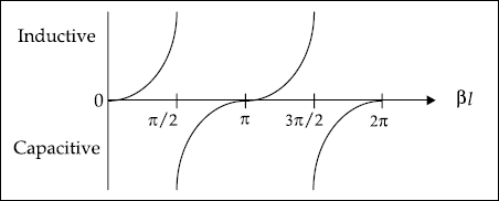
(a) Shorted load
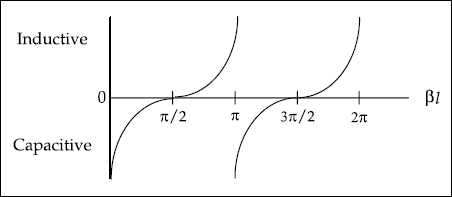
(b) Open circuited load
Fig. 7.7 Input impedance variation
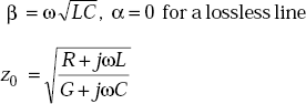
7.14 RF LINES
At radio frequencies,
|
ωL >> R |
|
ωC >> G |
Then, |
Z = R + jωL ≈ jωL |
|
Y = G + jωC ≈ jωC |
|
|
and |
|
|
|
As γ = α + jβ, α ≈ 0, ![]() , it is not enough if α is small compared to β. Hence let us consider,
, it is not enough if α is small compared to β. Hence let us consider,
For RF lines, the input impedance is
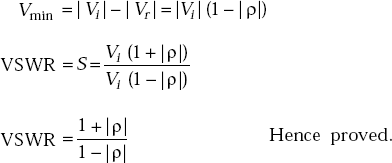
7.15 RELATION BETWEEN REFLECTION COEFFICIENT, LOAD AND CHARACTERISTIC IMPEDANCES
where |
ρ |
= |
reflection coefficient |
|
zL |
= |
load impedance |
|
z0 |
= |
characteristic impedance |
Proof For lossless RF lines, we have
Similarly,
At the load, (l = 0)
I at any point from load is
Load current, IL
But by definition, the reflection coefficient, ρ is
and
Dividing both sides by Vi, we get
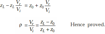
If |
zL |
= |
z0, ρ = 0 |
|
zL |
= |
0, ρ = −1 |
|
zL |
= |
∞, ρ = 1 |
|
zL |
= |
purely reactive, |ρ|= 1 |
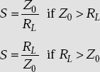
7.16 RELATION BETWEEN REFLECTION COEFFICIENT AND VOLTAGE STANDING WAVE RATIO (VSWR)
VSWR is defined as
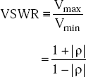
Proof We can write
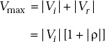
Similarly,
We can also write |ρ| as
When the line is terminated by purely resistive load,
7.17 LINES OF DIFFERENT LENGTH—  LINES
LINES
By selecting a terminated line of suitable length, it is possible to produce the equivalent of a pure resistance, inductance and capacitance or any desired combination thereof.
Equivalent circuits for shorted and open lines are shown in Table 7.3.
Table 7.3 Equivalent Circuits for Shorted and Open Lines
| Length of line | Equivalent circuit element | |
|---|---|---|
| Shorted line | Open line | |
Inductor |
Capacitor |
|
Tank circuit |
Series-resonant circuit |
|
Capacitor |
Inductor |
|
Series-resonant circuit |
Tank circuit |
|
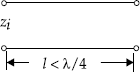
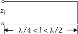
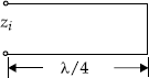
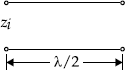
In Table 7.4, lines of different length with short and open ends along with their equivalent circuits are shown.
Table 7.4 Equivalent Circuit and Impedance
| Transmission line | Equivalent circuit | Input impedance |
|---|---|---|
|
|
zi = + jz0 tan βl |
|
|
zi = + jz0 cot βl |
|
|
zi = + jz0 tan βl |
|
|
zi = + jz0 cot βl |
|
|
|
|
|
|


7.18 LOSSES IN TRANSMISSION LINES
Losses in transmission lines are of three types:
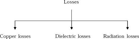
Copper Loss
These losses occur because of the following reasons:
- I2 R power loss This is due to dissipation as a result of heating in pure resistance. Its features are:
- Copper loss is small if there are no current loops, that is, the line should be properly terminated without producing standing waves.
- Copper loss is more if z0 is small. This is because, if z0 is low, current is high. If the current is high, copper loss is more.
- Skin effect Its features are:
- When an AC signal at high frequency is applied to the transmission lines, the current is confined to the surface (skin) of the conductors. This is known as skin effect. This effect reduces the cross-sectional area of the conductor with increase in frequency.
- Decrease in cross-sectional area increases the resistance.
- Increased resistance increases power losses.
- Crystallisation Its features are:
- Copper losses increase due to ageing of the transmission line. Losses are more when the line is subjected to high temperature, high winds and moisture. Moreover, bending of the line back and forth causes the line to become brittle and cracks appear. This effect is known as crystallisation of the conductors.
- Crystallisation increases resistance in the conductors which in turn increases copper losses.
Dielectric Losses
These losses exist due to improper characteristics of dielectric.
Salient features:
- These are due to 12 R power dissipation because of the heating of the solid dielectric material between conductors in transmission lines. These losses are proportional to the voltage across the dielectric.
- With increased frequencies, solid dielectric properties worsen and hence transmission lines with solid dielectrics have limited applications.
- Lines with air dielectric are used at high frequencies, as air dielectric loss is very small.
Radiation Losses
Salient features:
- These losses are high when the spacing between the lines is high as the transmission line acts as an antenna. Therefore, radiation losses are more in parallel-wire lines than in coaxial lines.
- At high frequency, I will be small and hence the transmission lines are not useful at high frequencies.
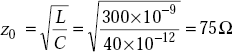
Problem 7.1 A transmission line with air as dielectric has z0 = 50 Ω and a phase constant of 3.0 rad/m at 10 MHz. Find the inductance and capacitance of the line.
Solution A line with air dielectric is lossless as σ = 0.
and
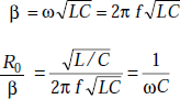
or,
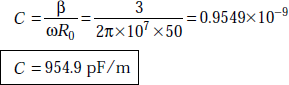
As
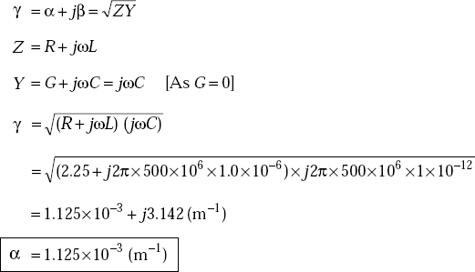
Problem 7.2 A lossy cable which has R = 2.25 Ω/m, L = 1.0 μH/m, C = 1pF/m, and G =0 operates at f = 0.5 GHz. Find the attenuation constant of the line.
Solution The propagation constant is given by
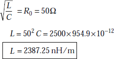
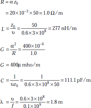
Problem 7.3 A transmission line in which no distortion is present has the following parameters: z0 = 50 Ω, α = 0.020 m-1, υ = 0.6υ0. Determine R, L, G, C and wavelength at 0.1 GHz.
Solution For a distortionless line the condition is
and
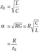
and hence
Problem 7.4 For a transmission line which is terminated in a normalised impedance zn, VSWR = 2. Find the normalised impedance magnitude.
Solution Normalised impedance, zn
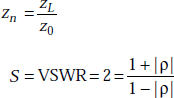
or,
We have
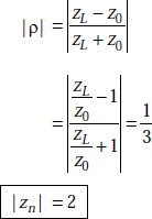
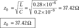
Problem 7.5 A lossless transmission line used in a TV receiver has a capacitance of 50 pF/m and an inductance of 200 nH/m. Find the characteristic impedance for sections of a line 10 metre long and 500 metre long.
Solution The characteristic impedance of a lossless transmission line is
The inductance, L of the line
For 10 m line,
|
L |
= |
200 × 10−9 × 10 = 2000 × 10−9 |
|
|
= |
2 × 10⁻⁶ H |
|
C |
= |
50 pF/m |
For 10 m line,
The characteristic impedance, z0
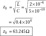
The inductance of 500 m line
|
L |
= |
200 × 10−9 × 500 |
|
|
= |
10,0000 × 10⁻⁹ |
|
L |
= |
10−4 H |
The capacitance of 500 m line
| C | = | 50 × 10−12 × 500 | |
| = | 25000 × 10−12 = 25 × 10−9 F |
The characteristic impedance, z0 of 500 m line
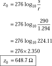
Problem 7.6 A two-wire open air line, whose diameter is 2.588 mm, is used in several applications. The wires are spaced at 290 mm between the centres. Find out the characteristic impedance of the line.
Solution Radius of the wire
Spacing between the wires is
The characteristic impedance of the two-wire open air line is
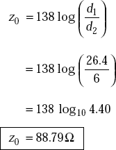
Problem 7.7 A copper coaxial line has an outside tubing of thickness 1.8 mm and its outside diameter is 30 mm. The thickness of the inner tubing is 1.0 mm and its outside diameter is 8 mm. Find the characteristic impedance of the line.
Solution Diameter of the outside conductor is
Diameter of the inner conductor is
For a coaxial cable, Z0 is
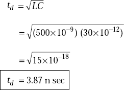
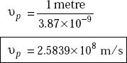
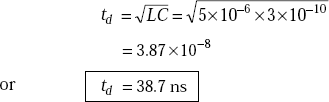
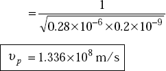
Problem 7.8 If a signal of 30 MHz is transmitted through a coaxial cable which has a capacitance of 30 pF/m and an inductance of 500 nH/m. (a) Find the time delay for a cable 1 m long, (b) propagation velocity, and (c) propagation delay over a cable length of 10 m.
Solution
- The time delay for 1 m long cable is
- Velocity of propagation,
- The inductance of 10 metre cable is
L = 500 × 10−9 × 10 = 5 × 10⁻⁶ H
The capacitance of 10 metre cable is
The time delay,
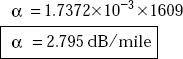
Problem 7.9 The attenuation coefficient of a transmission line is 0.2mNp/m. Find the attenuation coefficient in (a) dB/m (b) dB/mile.
Solution
- Attenuation coefficient in Np/m is
α = 0.2 × 10⁻³ Np/m
Attenuation coefficient, in dB/m is
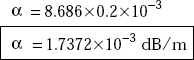
- 1 mile = 1609 m
The attenuation coefficient, α in dB/mile is
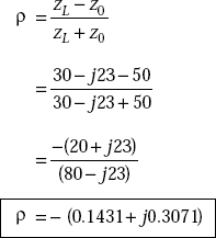
Problem 7.10 A lossless transmission line is terminated in a load impedance of 30 – j 23 Ω. Find the phase constant and the reflection coefficient of a line of length 50 m. Characteristic impedance, z0 = 50Ω. Wavelength on the line = 0.45 m.
Solution
|
zL |
= |
(30 − j23) Ω |
|
z0 |
= |
50 Ω |
|
λ |
= |
0.45 m |
|
l |
= |
50 m |
Phase constant,
Reflection coefficient,
Problem 7.11 A coaxial cable has z0 of 75 Ω and a capacitance of 70 pF/m. Find its inductance per metre. If the radius of the inner conductor is 0.292 mm and the relative permittivity of the dielectric is 2.3, determine the radius of the outer conductor.
Solution Radius of the inner conductor,
We have
or,
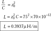
For a coaxial cable, z0 is also given by
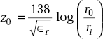
or,
where r0 = radius of the outer conductor.
Problem 7.12 A lossless transmission line of length 100 m has an inductance of 28μH and a capacitance of 20 nF. Find (a) propagation velocity (b) phase constant at an operating frequency of 100 kHz (c) characteristic impedance of the line.
Solution Length of transmission line,
Inductance of the line
Inductance/metre ![]()
Capacitance of the line = 20 nF
Capacitance per metre
Problem 7.13 The dielectric material between two conductors of a lossless coaxial cable has ∈r = 4 and μr = 1. Diameter of the inner conductor is 2 mm. Characteristic impedance of the 10 m long cable is 50Ω. Determine the diameter of the outer conductor of the coaxial cable.
Solution The expression for inductance and capacitance of a coaxial cable is
and

where |
μ |
= |
permeability = μ0 μr |
|
∈ |
= |
permittivity = ∈0∈r |
|
d0 |
= |
diameter of outer conductor |
|
di |
= |
diameter of inner conductor |
The expression for the characteristic impedance, z0 is
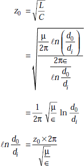
Here
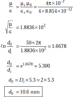
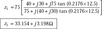
Problem 7.14 A transmission line is lossless and is 25 m long. It is terminated in a load of zL = 4o + j30Ω at a frequency of 10 MHz. The inductance and capacitance of the line are L = 300 nH/m, C = 40 pF/m. Find the input impedance at the source and at the mid-point of the line.
Solution The length of transmission line = 25 m.
Load impedance,
Inductance,
Capacitance,
Characteristic impedance,
Phase constant, β
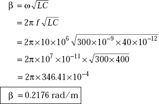
Input impedance at the source end is
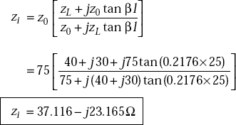
Similarly, input impedance at 12.5 m from source end is
7.19 SMITH CHART AND APPLICATIONS
Smith chart is a polar plot of the reflection coefficient in terms of normalised impedance, r + jx. In other words, it is a graphical plot of normalised resistance and reactance in the reflection coefficient plane.
It was designed by Phillip H. Smith in 1939.
Construction of Smith Chart
It is constructed within a circle of unit radius (| ρ | ≤ 1) as in Fig. 7.8.
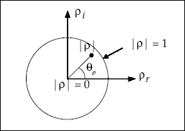
Fig. 7.8 Construction of Smith chart on unit circle
Smith chart provides the relation between reflection coefficient, ρ load, zL and characteristic impedance, z0. Here, the impedances are always normalised with respect to characteristic impedance,
|
|
or, |
ρ = |ρ| ∠θρ = ρr + jρi |
Smith charts are constructed in terms of normalised impedances (zL / z0) to avoid construction of one chart for each z0. Normalised load impedance is
or,
or,
and
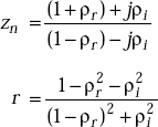
The Equations (7.8) and (7.9) are the equations of circles like
Equation (7.8) is known as r-circle and Equation (7.9) is known as x-circle.
The resistance circle has centre at ![]() and radius of
and radius of ![]() as in Fig. 7.9.
as in Fig. 7.9.
Fig. 7.9 r-circles
The reactance circle has centre at ![]() and radius
and radius ![]() as shown in Fig. 7.10.
as shown in Fig. 7.10.
Fig. 7.10 The reactance circles
Salient features of r and x-circles
- The centres of all r-circles lie on ρr -axis where ρr is the real part of the reflection coefficient. The centre straight line is called ρr axis.
- The r = 0 circle having unity radius and centre at the origin is the largest.
- The r-circles become progressively smaller as r increases from 0 to ∞ ending at the point (ρr = 1, ρi = 1) for open circuit.
- All circles pass through the (ρr = 1, ρi = 0) point.
- The centre of all x-circles lie on the ρr = 1 line.
- The x-circles for x > 0 (inductive reactance) lie above ρr -axis and those for x <0 (capacitive reactance) lie below the ρr -axis.
- The x = 0 circle becomes ρr -axis.
- X-circle becomes progressively smaller as | x | increases from 0 to ∞ ending at the point (ρr = 1, ρi = 0) for open circuit.
- All x-circles pass through the (ρr = 1, ρl = 0) point.
- The Smith chart consists of two sets of circles or arcs of circles. The complete circles lie on the centre line on the chart. These circles correspond to various
values of normalised resistance
 along the line.
 - The arcs of the circles on either side of the straight line correspond to various
values of normalised line reactance,

- The circles are orthogonal to each other.
- The perimeter of the outer rim of the chart is of
 length.
Applications of Smith Chart
It can be used to:
find the parameters of mismatched transmission lines
find normalised admittance from normalised impedance or vice-versa
find VSWR for a given load impedance
design stubs for impedance matchings
locate a voltage maximum on the line
find the input impedance of a transmission line.
7.20 STUBS
A stub is a piece of transmission line. It can be short circuited at the far end or open circuited. It has a pure reactance or susceptance. It is used to cancel out reactance or susceptance of a transmission line. In other words, it is used for impedance matching.
In general, shorted stubs are more frequently used since open ended stubs tend to radiate. The design parameters of stubs are (1) stub length and (2) stub distance from the load. The matching of transmission lines is done by the design of a single stub or a double stub.
Design of Single Stub Matching
The design consists of the following steps:
- Given zL and z0 of transmission line, normalise zL, or, find
zn = zL / z0 = r + jx
- Mark the point on the Smith chart where r-circle and x-arc intersect.
- Draw a circle with the radius equal to the distance from the centre of the chart to the point.
- Draw a straight line from this point through the centre of the chart to the other half of the chart, that is, travel around it through a distance of
 (or, straight through) to find the load admittance. As the stub is placed in parallel with the main line, it is easy to deal with admittances to make stub calculations.
 - Mark the point where the straight line intersects the circle drawn. This point gives the normalised admittance, (g + jb).
- Note the point where the circle cuts the centre straight line of the chart to the right side of the centre. Read the value of that point. It gives VSWR straight away.
- Note the point nearest to the load at which the normalised admittance is 1 ± jb. This is the point where ± jb intersects the r = 1 circle. Moreover, this is the point at which a stub, designed to tune out ± jb component, will be placed.
- Note the distance travelled round the circumference of the chart. This is the distance of the stub from the load.
- Move clockwise round the perimeter of the chart and find the point at which the susceptance tunes out ± jb susceptance of the line. For example, if the line admittance is 1 + jb, the required susceptance is – jb.
- Note the distance in wavelengths from ∞, j ∞ of the chart to the new point (Example: susceptance is – b). This gives the length of the stub required.
A typical stub is shown in Fig. 7.11.
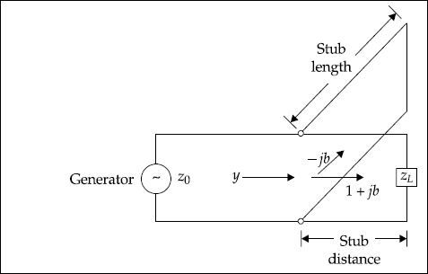
Fig. 7.11 Shorted stub connected to a transmission line
Problem 7.15 Find the input impedance of 75Ω lossless transmission line of length 0.1λ when the load is a short.
Solution Load impedance,
Characteristic impedance,
Length of the line = 0.1λ
The normalised load impedance is
Steps Involved
- Start from the point Psc at the left of the rim of the chart. Psc is intersection of r = 0, x = 0.
- Move clockwise from Psc through the perimeter of the chart by 0.1λ towards generator. Mark point Ps (Refer Fig. 7.12).
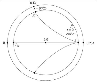
Fig. 7.12 Lossless transmission line where load is short
- At Ps, r = 0 and x = 0.725, that is, zin = normalised input impedance = 0 + j 0.725.
- The input impedance,
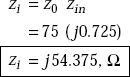
Analytical method The expression for zi (for lossless line) is
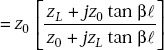
If
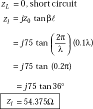
Problem 7.16 Find the input impedance of a 75Ω lossless transmission line of length (0.1λ) if it is terminated in open circuit.
Solution
|
l |
= |
0.1λ |
|
zL |
= |
∞ (open) |
|
z0 |
= |
75 Ω |
The expression for input impedance is
If the load is open circuit,
Smith chart method
- Start from the point Poc at the right of the rim of the chart.
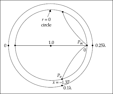
Fig. 7.13 Lossless transmission line terminated in open circuit
- Move clockwise from Poc through the perimeter of the chart by 0.1λ towards generator. Mark point Po (Refer Fig. 7.13).
- At P0 r = 0, x = −1.37, that is, the normalised input impedance.
zin = 0 − j1.37
- Input impedance,
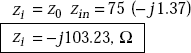
Problem 7.17 A transmission line of length 0.40λ has a characteristic impedance of 100Ω and is terminated in a load impedance of 200 + j180Ω. Find the
- voltage reflection coefficient
- voltage standing wave ratio
- input impedance of the line
Solution The data is
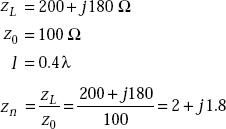
(a)
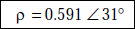
- Refer Fig. 7.14. Locate the point 2.0 + j 1.8 on the Smith chart. It is represented by A.
- Draw a circle of radius equal to OA. This OA is | ρ | and it is equal to 0.591.
- Draw a straight line OA and extend it to B. Read 0.207 in wavelength towards the generator.
- The phase angle of the reflection coefficient is given by
(0.250 − 0.207) × 4π = 0.043 × 4π = 31°
Hence the reflection coefficient is
(b) The reflection coefficient |ρ| = 0.591 circle meets the positive real axis opoc at r = 4, that is,
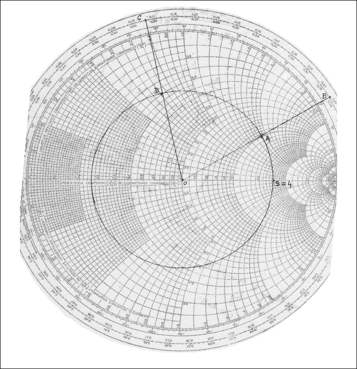
Fig. 7.14
(c) To determine zi,
- Move B at 0.207 by a total of 0.40 wavelengths towards generator. Movement is made from 0.40 to 0.50 to 0.107. This point is represented by C.
- Draw a line joining the centre and point C. This intersects circle at D.
- Read the values of r and x at this point, that is, r = 0.4 and x = 0.72.
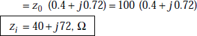
Normalised input impedance
Input impedance
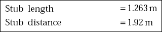
Problem 7.18 Design a stub to match a transmission line which is connected to a load impedance of zL = (450 – j 600) Ω. The characteristic impedance of the line is 300 Ω. The operating frequency is 20 MHz.
Solution
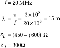
- The normalised load impedance is
- Identify the point of intersection in Fig. 7.15, r = 1.5 and x = −2.0.
- Draw a circle with a radius of OA. It cuts the centre line at 4.8. Therefore, VSWR = 4.8.
- Draw a line OA and extend it to B. This point, B represents normalised admittance, yn, that is, yn = 0.22 + j 0.35.
- The drawn circle cuts r = 1 circle at C. This point corresponds to 1 + j 1.7.
- The distance of D to E on the rim of the chart is the stub distance from the load.
The stub distance
=
(0.181 0.053) λ = 0.128λ
=
0.128 × 15 = 1.92 m
- As the load has a susceptance of + j1.7, the stub is required to provide a susceptance of – j 1.7. Therefore, mark a point by moving clockwise on the lower half of the chart. It is marked by F. Its distance from the short circuit admittance point is given by
0.3342 − 0.25 = 0.0842λ
Stub length
= 0.0842λ
= 0.0842 × 15 = 1.263 m
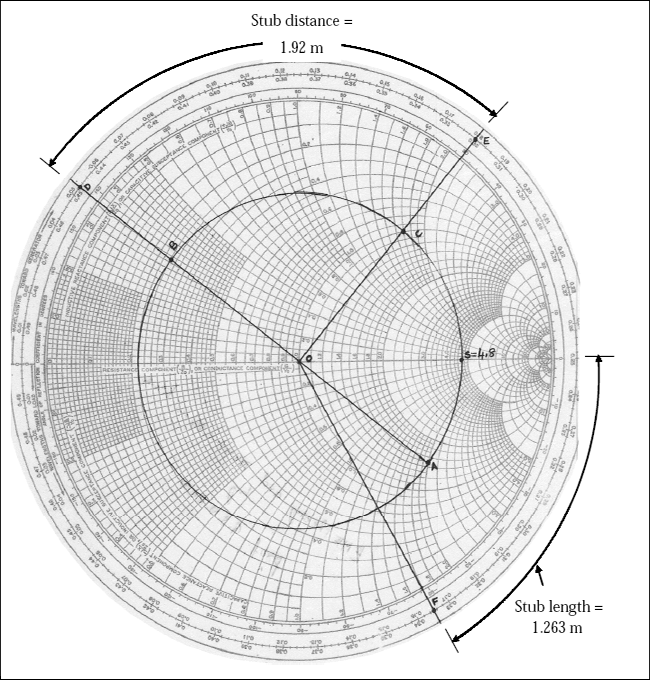
Fig. 7.15
The designed stub parameters are:
7.21 DOUBLE STUBS
For the design of any device, it is convenient to have more parameters in designer’s control for more freedom. For this purpose, to match the load with the transmission line, a second stub of adjustable position is included. A typical double stub is shown in Fig. 7.16.
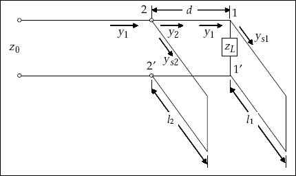
Fig. 7.16 Double stub transmission line
It is also possible to use a triple stub tuner for more design convenience.
In single stub matching the stub is placed on the line at a specified point. Its location varies with zL and frequency. This creates some difficulties as the specified point may occur at an undesirable location. In such cases, double stubs are used. Here the distance between them is fixed such as ![]() and so on and the lengths of the two stubs are adjusted to match the load.
and so on and the lengths of the two stubs are adjusted to match the load.
Design Methodology
Step 1 |
Fix the distance between the two stubs and keep stub 1 at the location of the load. |
Step 2 |
Draw the circle corresponding to the normalised conductance, g = 1. |
Step 3 |
Obtain the normalised distance of |
Step 4 |
Rotate the circle in anticlockwise direction by |
Step 5 |
Locate yL = gL + jbL. |
Step 6 |
Draw g = gL circle. This intersects the rotated g = 1 circle at one or two points where yL = gL + jb1. |
Step 7 |
Locate the corresponding y2 points on the g = 1 circle. y2 = 1 + jb2. |
Step 8 |
Find the stub length l1 between the points representing yl and yL. |
Step 9 |
Find the stub length l2 from the angle between the point representing –jb2 and psc. |
The stub distances from the load need not be found as d is fixed.
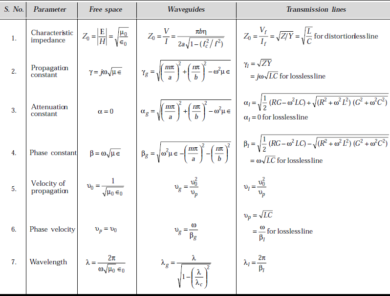
In Table 7.5 given on the next page, propagation characteristics of EM waves in free space, in waveguides and in transmission lines are compared.
Table 7.5 Comparison between the Propagation Characteristics of EM Waves in Free Space, Waveguides and Transmission Lines
POINTS/FORMULAE TO REMEMBER
- Transmission lines transfer information from one point to another.
- They are characterised by the presence of distributed constants R, L, G and C.
- Transmission lines are used as impedance matching devices, stubs.
- Coaxial cables are used to connect TVs to antennas.
- Microstrips are used in integrated circuits.
- Twisted pairs and coaxial cables are used in computer networks such as Ethernet.
- Optical fibres are characterised by negligible attenuation and infinite bandwidth.
- Equivalent circuit of a uniform transmission line is shown in Fig. 7.17.
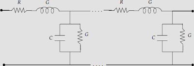
Fig. 7.17
- The characteristic impedance of a pair of transmission lines is

- The propagation constant of a transmission line is

- For a lossless transmission line
- For a distortionless transmission line,

- For a lossless and distortionless transmission line,
 .
. - Loading of transmission lines is the introduction of inductance in series with the line.
- Input impedance of transmission line is
 .
. - Input impedance of a lossless transmission line is
 .
. - For a matched line Zi = Z0.
- For RF lines,
 .
. - For RF lines, the input impedance is
 .
. - The reflection coefficient,
 .
. - VSWR

- VSWR varies between 1 and ∞.
- For resistance terminated load,
- The losses in transmission lines are due to copper, dielectric and radiation.
- Smith chart is useful to measure transmission line parameters.
- The design parameters of a single stub are its length and its distance from the load end.
- Velocity elocity of propagation in lossless line is
 .
. - VSWR is defined as
 .
. - Characteristic impedance is defined as
 .
. - Reflection coefficient is defined as
 .
.
OBJECTIVE QUESTIONS


Answers
1. Yes |
2. Yes |
3. Yes |
4. Yes |
5. Yes |
6. Yes |
7. Yes |
8. Yes |
9. No |
10. No |
11. Yes |
12. Yes |
13. Yes |
14. Yes |
15. Yes |
16. No |
17. Yes |
18. Yes |
19. Yes |
20. TEM wave |
21. Two or more conductors
22. If the conductors are separated by the same dielectric, if they have same cross-sectional area along the length of the line and if they have same dimensions
23. A few mm
24. Smith chart
25. If the conductors have σ = ∞ and if the dielectric between the conductors has σ = 0
26. z0 tanh rl
27. ![]()
28. zi = zL
29. z0 changes at the point
30. ![]()
31. ![]()
32. 1 + ρ
33. ![]()
34. A piece of transmission lined
35. One
36. ![]()
37. The ratio
38. The time taken for the wave to travel from one end to the other
39. ![]() l = length of line, u is the velocity of propagation of the wave
l = length of line, u is the velocity of propagation of the wave
40. 1/3
41. ![]()
42. ![]()
43. ![]()
44. Lattice diagram
45. A time-distance diagram
46. PCBs
47. ![]()
48. ![]()
49. ![]()
50. ![]()
51. α + jβ
MULTIPLE CHOICE QUESTIONS
- If the load impedance in a transmission line is 100 + j200Ω and characteristic impedance is 100Ω, the normalised load impedance is
- 1 + j 2Ω
- 10,000 + j 20,000Ω
- 1 + j 200Ω
- 100 + j 2Ω
- If the normalised load impedance of a transmission line is 3 + j 4Ω, the normalised admittance is
- 0.6 − j 0.8 mho
- 1 − j 1.0 mho
- 1 + j 1.0 mho
- 0.6 − 0.8 mho
- If z0 = 50Ω, zL = 50 + 100j for a quarter wave transmission line, its input impedance is
- If the load impedance of one half-wavelength is 50 + j150Ω, its input impedance is
- 50 − j150Ω
- 50 + j 150Ω
- 50 + j 100Ω
- 1 + j 1.5Ω
- If the load impedance in a transmission line is zL and z0 is the characteristic impedance, reflection coefficient is
- If reflection coefficient in a transmission line for a given load is 0.5 + j 0.5, VSWR is
- 1
- ∞
- 2
- − ∞
- If maximum and minimum voltages on a transmission line are 4 V and 2 V respectively, VSWR is
- 0.5
- 2
- 1
- 8
- If the sending voltage and currents on a transmission line are 200 V and 2 amp for a given load the input impedance is
- If the voltage and current at the receiving end of a transmission line for a given load are 3.0 V and 200 mA respectively, the load impedance is given by
- 600 Ω
- 150 Ω
- 1500 Ω
- 15 Ω
- A lossless transmission line characterised by a distributed inductance of 300 nH/m and capacitance of 50 PF/m operates at no load. Its characteristic impedance is
- 60 Ω
- 600 Ω
- 77.45 Ω
- 774.5 Ω
- The velocity of propagation of a wave along a transmission line of length 100 m is 2.8 × 10⁸m/s. The delay on the transmission line is
- 3.57 ns
- 357 ns
- 0.357 ns
- 2.8 μ s
- A 100 km long transmission line has an inductance of 27 mH. Its distributed inductance per metre is
- 27 mH
- 2.7 μ H
- 0.27 μ H
- 27 μ H
- A 100 km long transmission line has a capacitance of 20 nF. Its distributed capacitance per metre is
- 0.20 PF
- 20 PF
- 20 nH
- 0.20 nF
- A 100 m long lossless transmission line is operating at 100 kHz. If the velocity propagation of the wave on the line is 1.4 × 10⁸ m/s, the propagation constant is
- 4.487 rad/m
- 4.487 m rad/m
- 44 m rad/m
- 0.4487 m rad/m
- A voltage of 2 cos 105 t volts is applied to a parallel plate transmission line. If the plate separation is 2 mm, the electric field between the plates at the source end is
- 1,000 cos 105 tV/m
- cos 105 tV/m
- 10 cos 105 tV/m
- cos 105 tmV/m
- A sinusoidal voltage with a wavelength of 100 cm is applied to a transmission line along which the velocity of propagation of the wave is 2.9 × 10⁸ m/s. The frequency of the source is
- 2.9 MHz
- 2.9 GHz
- 0.29 GHz
- 0.29 MHz
- If the magnitude of the reflection coefficient on a transmission line for a given load is 1/3, VSWR is
- A 50Ω transmission line is connected to a load impedance yielding a VSWR of unity. The load impedance is
- 50 Ω
- 100 Ω
- 1 Ω
- 0 Ω
- A load impedance of 100W is connected to a 50W line. VSWR of unity is obtained by connecting
- another 50 Ω in series with zL
- another 50 Ω in parallel to zL
- another 100 Ω in parallel to zz
- another 100 Ω in series with zL
- If the reflection coefficient at a point on a transmission line is − 0.5, the transmission coefficient is
- 0.5
- − 0.5
- 1.0
- 0
Answers
1. (a) |
2. (a) |
3. (a) |
4. (b) |
5. (a) |
6. (b) |
7. (b) |
8. (a) |
9. (b) |
10. (c) |
11. (b) |
12. (c) |
13. (a) |
14. (b) |
15. (a) |
16. (c) |
17. (b) |
18. (a) |
19. (c) |
20. (a) |
EXERCISE PROBLEMS
- A parallel wire transmission line is made of copper. The separation between the wires is 1.0 m in air. The conductor radius is 2.0 mm. Find L, C and G.
- A copper parallel wire transmission line operates at 1 MHz. For copper μc = μ0 , ∈c = ∈0 , σc = 5.8 × 10⁷ mho/m. The radius of the wire, a = 2.0 mm. Find Rdc and Rac
- A transmission line is characterised by
R = 10-2 Ω/m, G = 1.0μmho/m and C = 1.0 μF/m.
Determine the characteristic impedance if the operating frequency is 1.59 kHz.
- A transmission line has
R = 0.01Ω/m, G = 1.0μ mho/m, L = 10μ H/m, C = 1.0μ F/m.
Find the attenuation constant, phase constant and phase velocity.
- A telephone line of 100 km has R = 4Ω/km, L = 3 mH/km, G = 1.0μ mho/km,C = 0.015μ F/km. It operates at 796 Hz and is connected to a load impedance of 200Ω. Find the series impedance, shunt admittance, characteristic impedance and reflection coefficient.
- A 100 km telephone line has R = 4Ω/km, L = 3 mH/km, G = 1.0μ mho/m and C = 15 nF/m. It operates at f = 796 Hz. Find the attenuation and phase constants.
- A coaxial cable has air dielectric. Its outer radius is 2.0 mm and inner radius is 1.0 mm. Find its characteristic impedance.
- A pair of transmission lines are separated by 1.0 m and each wire has a radius of 1 cm. Find z0.
- A uniform transmission line operating at 10 kHz has z0 of 50Ω and propagation constant, γ = (0.1 + j 0.1) m-1. Find R and L.
- A uniform transmission line operating at 1 kHz has z0 = 75W and a propagation constant of (0.1 + j 0.2) m-1 . Find G and C.
- For a uniform transmission line, the open and short circuit impedances are given by zoc = 50 + j 25Ω, zsc = 60 − j 20Ω. Find z0 of the line.