Chapter 2
Electrostatic Fields
Electrostatic fields are produced by charges at rest.
The main objective of this chapter is to provide detailed concepts of electrostatics. They include:
- applications of electrostatics
- charge distributions
- Coulomb’s law, applications and limitations
- Gauss’s law, applications and limitation
- potential functions
- Poisson’s and Laplace’s equations
- conductors, dielectrics and capacitors
- energy stored in electrostatic fields and capacitors
- fields in dielectrics and boundary conditions
- solved problems, points/formulae to remember, objective and multiple choice questions and exercise problems.
2.1 INTRODUCTION
Electrostatic fields are also called static electric fields or steady electric fields. These fields are not variant with time. They are produced by static charges or charge distributions. These fields have a wide range of applications.
In this chapter, the important laws, theorems and equations, with their applications are presented to provide a thorough understanding of electrostatics. The important areas are Coulomb’s and Gauss’s laws, Stoke’s and divergence theorems and Poisson’s and Laplace’s equations.
2.2 APPLICATIONS OF ELECTROSTATIC FIELDS
Electrostatic fields are used
- in cathode ray oscilloscopes to obtain the electron beam deflection
- in ink-jet printers to obtain speed of printing and quality of print
- to sort out minerals in ore separators, to sort out seeds in agriculture and for spraying plants and trees
- in electrostatic generators
- to produce potential
- to produce force on charges for their mobility
- in electric power transmission
- in lightning protection
- to measure moisture content
- to spin cotton
- in field-effect transistors
- in capacitors
- in LCDs
- in touch pads
- in capacitance keyboards
- in fast baking of bread
- in ECGs, EEGs, ERG, EMG, EOG in medical applications
- in spray painting
- in electrodeposition
- in electrochemical machining
- X-ray machines
- computer peripherals
2.3 DIFFERENT TYPES OF CHARGE DISTRIBUTIONS
Charges at rest produce electrostatic field. The charges are basically of two types: positive and negative.
Properties and Functions of Charges
- Charge is conserved. It can neither be created nor destroyed.
- Charge is quantisised that is, it comes in discrete quantities and in integer multiples of the basic unit of charge. Electron charge or proton charge is the basic charge.
- When a charge is accelerated, electromagnetic field is produced. A fraction of the field is detached and propagates at the speed of light. The detached field carries energy, momentum and angular momentum. This is called electromagnetic radiation.
- Charges are surrounded by electric and magnetic fields.
- A charge experiences a force in the presence of a field.
- Charges mediate the integration of fields.
Charge density and charge distribution indicate the same property. In practice, there are four types of charge distributions.
(i) |
Point charges, Q (Coulomb) These are the charges which do not occupy any space, that is, the volume of the point charge is zero. For example, an electron is considered to be a point charge and has a charge of 1.6 × 10⁻¹⁹ Coulombs (C). |
(ii) |
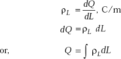
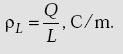
Line charge distribution, ρL (c/m) This is a charge distribution in which the charge is distributed along a line like a filament, that is, this has only length but no width or breadth. ρL is defined as the charge per unit length, that is, |
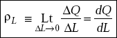
where ΔQ is small charge, ΔL is small length, dQ is differential charge and dL is differential length.
Sometimes, ρL is simply considered as Q/L.
An example is the electron beam in CRT.
Problem 2.1 If there is a charge of 10μC over a filament length of 0.5 m, find its line charge density.
Solution Here, Q = 10μC = 10 × 10–6 C
L = 0.5m
Line charge density, ρL = Q/L = 10 / 0.5 = 20 μC / m
(iii) |
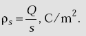
Surface charge distribution, ρs (c/m2) When a charge is confined to the surface of a conductor, it is said to be surface charge distribution. Such a surface has both length and width but no breadth. |
Surface density is defined as the charge per unit area, that is,
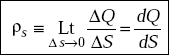
where ΔS is small area and dS is differential area.
Sometimes, ρs is simply considered as Q/S.
An example is the conductor surface of a capacitor.
Problem 2.2 If there is a total charge of 10 pC over a surface area of 0.2 m2, find the surface charge density.
Solution Here, Q = 10 pC = 10 × 10–12C
S = 0.2 m2
Surface charge density, ρs = Q/ S = (10 × 10–12)/0.2
= 50pC/m2
(iv) |
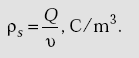
Volume charge distribution, ρv (c/m3) Volume charge density is defined as the charge per unit volume, that is, |
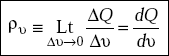
where dv is differential volume.
Sometimes, ρv is simply considered as ![]()
Examples are ionospheric region, electron cloud in vacuum tube.
Problem 2.3 If there exists a total charge of 12 nC in a spherical volume of 0.1 m3, find the volume charge density.
Solution Here Q = 12nC = 12 × 10 –9C
v = 0.1 m3
The volume charge density,
ρv = Q / v
= 12 / 0.1
= 120 nC / m3
2.4 COULOMB’S LAW
Charles Augustin De Coulomb (1736–1806) was a French physicist. After conducting several experiments on charged bodies, he concluded that there exists a force between them. He formulated a law known as Coulomb’s law.
The law appears in the following forms:
- Gaussian form
Force,

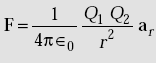
- SI form
Force,
- Heavside-Lorentz form
Force,
Law statement Coulomb’s law states that there exists a force between charged bodies and it is:
- Proportional to the product of the two charges,
- Inversely proportional to the square of the distance between the charges. The force also depends on the medium in which the charges are located.
The force is a vector quantity and it is attractive if the charges are unlike and repulsive if the charges are alike. It acts along the straight line joining the two charges.
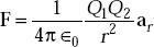
Mathematically, Coulomb’s law is given by,
where |
k = a constant of proportionality |
|
|
Q1, Q2 are two point charges (C)
|
= |
force between the charges (Newton) |
r |
= |
distance between the charges (m) |
∈ |
= |
permittivity of the medium in which the charges are located (F/m) |
|
= |
∈0∈r |
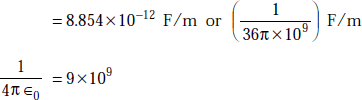
∈0 |
= |
permittivity of vacuum or free space |
|
|
|
∈r |
= |
relative permittivity of the medium with respect to free space (has no unit) |
|
= |
1 for free space |
k in free space
|
|
ar |
= unit vector along the line joining the two charges |
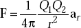
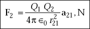
The force on Q2 due to Q1 in free space is written in the form of
where,
∈0 = permittivity of free space
The force on Q1 due to Q2 is
Problem 2.4 If Q1 and Q2 are two point charges and are located at r1 and r2 respectively in free space, find (a) the force on Q2 due to Q1, (b) the force on Q1 due to Q2.
Solution |
Q1 = first charge |
|
Q2 = second charge |
|
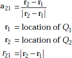
r1 = location of Q1 |
|
r2 = location of Q2 |
Distance vector along the line joining two charges,
The magnitude of r21 is
The direction of ![]()
- The force on Q2 due to Q1
- The force on Q1 due to Q2,
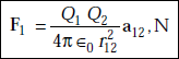
Here |
r12 = r1 − r2 = −(r2 − r1) = −r21 |
|
r12 = r21 = |r1 − r2| = |r2 − r1| |
|
a12 = −a21 |
|
F1 = −F2 |
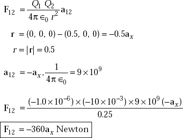
Problem 2.5 A charge of Q1 = –1.0μC is placed at the origin of a rectangular coordinate system and a second charge, Q2 = –10 mC is placed on the x-axis at a distance of 50 cm from the origin. Find the force on Q1 due to Q2 if they are in free space.
Solution |
Q1 = –1.0μC at (0, 0, 0) |
|
Q2 = –10 mC at (0.5, 0, 0) |
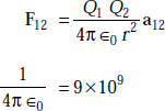
By Coulomb’s law,
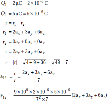
Problem 2.6 A point charge, Q1 = 2 μC is at (2, 3, 6) and another charge, Q2 = 5 μC is at (0, 0, 0) in free space. Find the force on Q1 due to Q2.
Solution We have
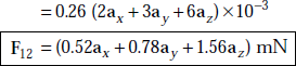
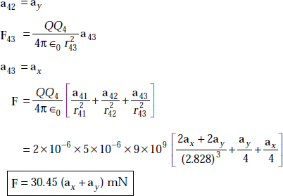
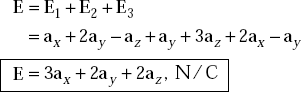
Problem 2.7 Three equal point charges of 2μC are in free space at (0, 0, 0), (2, 0, 0) and (0, 2, 0), respectively. Find net force on Q4 = 5μC at (2, 2, 0).
Solution
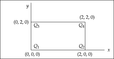
Fig. 2.1 Location of charges
|
Q1 |
= |
Q2 = Q3 = 2μC =Q |
|
Q4 |
= |
5μC |
|
r1 |
= |
(0, 0, 0) |
|
r2 |
= |
(2, 0, 0) = 2ax |
|
r3 |
= |
(0, 2, 0)= 2ay |
|
r4 |
= |
(2, 2, 0)= 2ax + 2ay |
|
r41 |
= |
r4 − r1 = 2ax + 2ay |
|
r42 |
= |
r4 − r2 = 2ax + 2ay − 2ax = 2ay |
|
r43 |
= |
r4 − r3 = 2ax + 2ay − 2ay = 2ax |
|
r41 |
= |
|
|
r42 |
= |
2, r43 = 2 |
The net force on Q4 due to Q1, Q2, Q3 is
Problem 2.8 Two charges Q1 = 2μC and Q2 = 5μC are located at (–3, 7, –4) and (2, 4, –1), respectively. Determine the force on Q2 due to Q1 and the force on Q1 due to Q2.
Solution The force on Q2 due to Q1 is given by
where
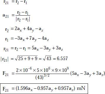
Now the force on Q1 due to Q2
2.5 APPLICATIONS OF COULOMB’S LAW
Coulomb’s law is used to:
- find the force between a pair of charges
- find the potential at a point due to a fixed charge
- find the electric field at a point due to a fixed charge
- find the displacement flux density indirectly
- find the potential and electric field due to any type of charge distribution
- find the charge if the force and the electric field are known.
2.6 LIMITATION OF COULOMB’S LAW
It is difficult to apply the law when charges are of arbitrary shape. Here, the distance, r cannot be determined accurately as the centres of arbitrarily shaped charged bodies cannot be identified accurately.
2.7 ELECTRIC FIELD STRENGTH DUE TO POINT CHARGE
Electrostatic field is produced by a charge at rest. It is defined by Coulomb’s law. Electric field strength or electric field intensity or electric field indicate the same property in this book.
Definition 1 Electric field due to a charge is defined as the Coulomb’s force per unit charge. It is a vector and has the unit of Newton per Coulomb or volt per metre, that is,
where F is Coulomb’s force, Newton and Q is charge, Coulomb.
Definition 2 Electric field is also defined as a negative gradient of a potential due to a charge, that is,
where V is potential due to the charge, volts.
Let |
Qf = fixed point charge, C |
|
Qt = test point charge, C |
|
rf = location of fixed charge |
|
rt = location of test charge |
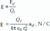
Then the force on Qt due to a fixed charge in free space, Qf is given by
The electric field, E at the location of Qt due to Qf is defined as the ratio of force on Qt due to Qf and the test charge, Qt, that is,
If there are N point charges, the field at a point is the vectorial sum of fields due to N charges, that is,
2.8 SALIENT FEATURES OF ELECTRIC INTENSITY
- It has units of Newton/Coulomb or volts/metre.
- It is a vector.
- It has both direction and magnitude.
- Its direction is the same as that of Coulomb’s force.
- Its magnitude depends on the magnitude of Coulomb’s force and the charge on which the force is acting.
- It depends on the medium.
- It depends on the permittivity of the medium.
- It depends on the distance of the charge from another charge which produces Coulomb’s force.
- It depends on the location of the charges.
- It originates from a positive charge and terminates on a negative charge.
- When a unit charge at a distance is moved around a fixed charge, the field lines and force appear as in Fig. 2.2.
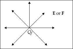
Fig. 2.2 Coulomb’s force and electric field
Problem 2.9 If Coulomb’s force, F = 2ax + ay + az N, is acting on a charge of 10C, find the electric field intensity, its magnitude and direction.
Solution Force,
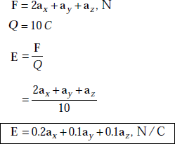
The magnitude of E is
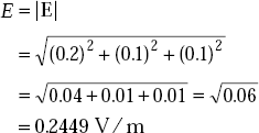
The direction of E is
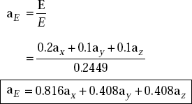
Problem 2.10 If a charge of 2μC is located at P1 (1, 0, 0) and another charge of 1 μC is located at P2 (0, 1, 0) in free space, find the electric field at P2.
Solution Let
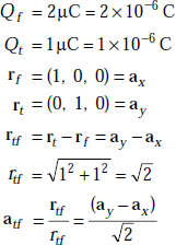
Electric field strength at P2 is
As
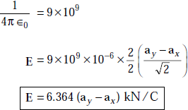
Problem 2.11 There are three charges which are given by Q1 = 1μC, Q2 = 2μC and Q3 = 3μC. The field due to each charge at a point, P in free space is ax + 2ay – az, ay + 3az and 2ax – ay N/C. Find the total field at the point, P due to all the three charges.
Solution The field, E1 at P due to Q1 (1μC)
The field, E2 due to Q2 (2μC)
The field, E3 due to Q3(3μC)
The total field at P,
Problem 2.12 A charge, Q1 = –10nC is at the origin in free space. If the x-component of E is to be zero at the point (3, 1, 1), what charge, Qt should be kept at the point (2, 0, 0)?
Solution Consider Fig. 2.3.
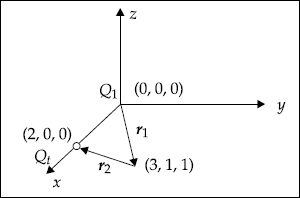
Fig. 2.3
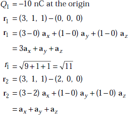
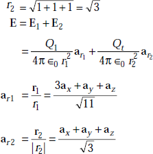
E at (3, 1, 1)
If Ex is to be zero, we should have
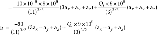
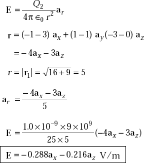
Problem 2.13 Two point charges Q1 = 5.0C and Q2 = 1.0nC are located at (–1, 1, – 3) m and (3, 1, 0) m, respectively. Determine the electric field at Q1.
Solution |
Q1 = 5.0 C is at (–1, 1, –3) m |
|
Q2 = 1.0 nC is at (3, 1, 0) m |
Electric field, E at Q1 (–1, 1, –3) m is
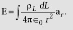
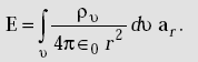
2.9 ELECTRIC FIELD DUE TO LINE CHARGE DENSITY
By definition, line charge density is given by
Here, Q is the total charge.
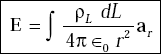
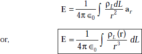
But electric field due to Q at a distance of r is given by
Problem 2.14 If a fine filament carries a uniform charge distribution of ρL c/m, find the electric field at a point, P2 (x1, y1, z1).
Solution Consider a differential length, dL on the line carrying the uniform charge. Let it be at a point P1 (x2, y2, z2) on the line.
The position P1 = r1 = x1ax + y1ay + z1az
The position P2 = r2 = x2 ax + y2 ay + z2az
r |
= |
r2 − r1 |
|
= |
(x2 − x1) ax + (y2 − y1) ay + (z2 − z1) az |
|r| |
= |
r =|r2 − r1| |
|
|
|
The electric field strength at P2 is
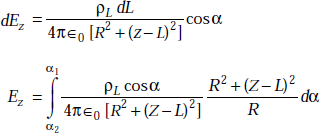
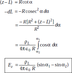
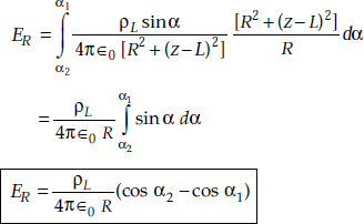
Problem 2.15 Find out electric field due to a uniformly charged short line (refer Fig. 2.4).
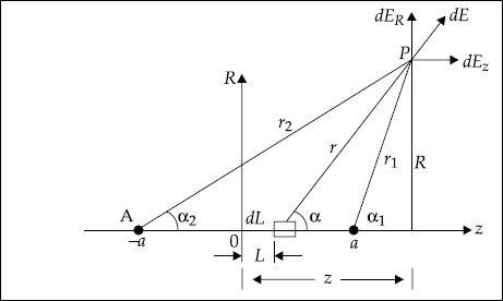
Fig. 2.4 Field due to a finite length of line charge
Solution It may be noted that there exists symmetry with the line charge along z-axis. Assume that the origin is at the centre of the line.
Consider dL at a distance of L from the origin. The magnitude of the charge, dQ of dL length is given by
Now |
|
|
|
or,
|
|
and ![]()
and
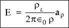
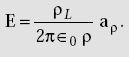
2.10 ELECTRIC FIELD STRENGTH DUE TO INFINITE LINE CHARGE
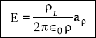
The electric field due to a uniform infinite line charge is given by
Proof For a line charge extending from –∞ to ∞ along z-axis, the electric field does not vary with z when ϕ and ρ are constants. It also does not vary with ϕ when z and ρ are constants due to symmetry.
The position of infinite line charge is shown in Fig. 2.5.
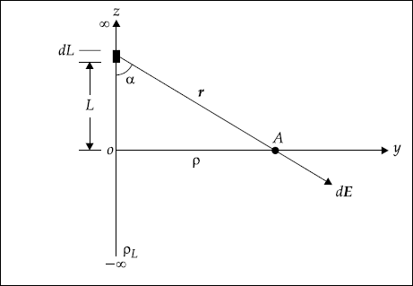
Fig. 2.5 Infinite line charge
Consider a differential length, dL along the line charge. Let it be at a distance of L from the origin. By definition, ![]()
The charge dQ of dL = ρL dL.
Consider a point A on y-axis at a distance of ρ from the origin. Let the field at A due to dQ be dE.
From Coulomb’s law
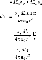
Here, ![]()
So,
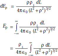
Put |
L = ρ tan θ |
|
dL = ρ sec2 θ dθ |
Now
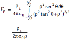
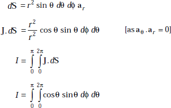
As Ez = 0 due to symmetry, the field strength is given by
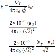
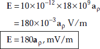
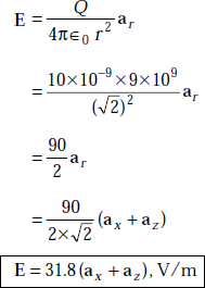
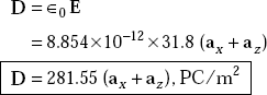
Problem 2.16 A charge density of ρL = 10 PC/m is uniformly distributed along an infinite line. Determine electric field at a point ![]() .
.
Solution The field at ![]() is
is
where
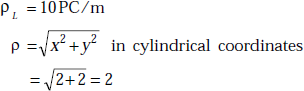
But ![]()
or ![]()
So,
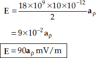
Problem 2.17 Find E at (2, 0, 2) if a line charge of 10 PC/m lies along the y-axis.
Solution We have ![]()
where
or,
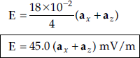
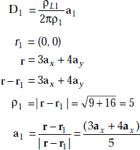
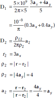
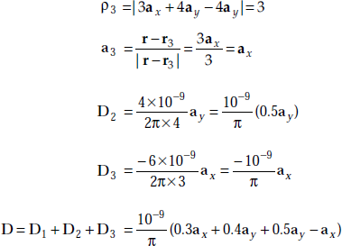
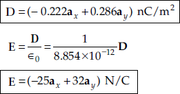
Problem 2.18 Three parallel line charges, ρL1 = 5 nC/m, ρL2 = 4 nC/m and ρL3 = –6 nC/m are located at (0, 0), (3, 0) and (0, 4) m, respectively. Find D and E at (3, 4).
Solution We have
ρL1 = 5 nC/m at (0,0)
ρL2 = 4 nC/m at (3, 0)
ρL3 = –6 nC/m at (0, 4)
D = D1 + D2 + D3
where
or,
or,
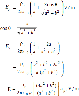
Problem 2.19 Three infinitely long lines charged uniformly are parallel to the z-axis. They are separated by a distance of b m. The charge density of each is ρL = 2.0 PC/m. Find the electric field E at a point P on the y-axis at y = a m. If a = b = 1 m, what is the electric field, E?
Solution Consider Fig. 2.6.
Expression for the electric field at a distance of P due to an infinitely long charged line, E is
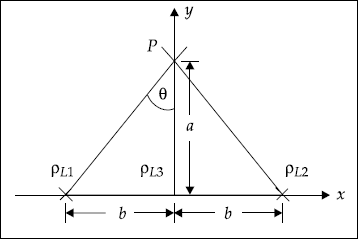
Fig. 2.6 A system of line charges
Ey1 at the point P due to ρL1
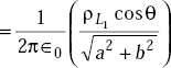
Ey3 at the point P due to ρL3
Ey2 at the point P due to ρL2
As ρL1 = ρL2 = ρL3 = ρL
Total
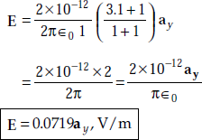
If a = b = 1m, ρL = 2.0 PC/m
Problem 2.20 An infinite length of uniform line charge has ρL = 10 PC/m and it lies along the z-axis. Determine the electric field E at (4, 3, 3) m.
Solution In cylindrical coordinates,
Due to symmetry, E is constant with z. Hence
or,
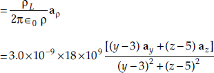
Problem 2.21 An infinitely long uniform line distribution of ρL = 3.0 nC/m is at y = 3, z = 5. Determine E at (a) (0, 0, 0), (b) (0, 2, 1), (c) (3, 2, 1).
Solution ρL = 3.0 × 10⁻⁹ C/m is at (x, 3, 5).
Let us take a general point (x, y, z). Then the radial vector from the location of ρL, that is, (x, 3, 5) to (x, y, z) is
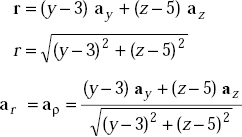
E at (x, y, z)
- E at (0, 0, 0)
- E at (0, 2, 1)
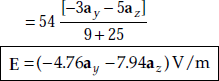
- E at (2, 3, 1)
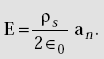
2.11 FIELD DUE TO SURFACE CHARGE DENSITY, ρs (C/m2)
Field due to surface charge density,
Consider an infinitely charged sheet lying in x-y plane. Assume that the sheet is uniformly charged.
Consider a strip of a differential width of dx as in Fig. 2.7.
The sheet extends from – ∞ to ∞ in both x and y directions. It is obvious that the field does not vary with x or y due to symmetry. Now, there is only z-component.
By definition, ![]()
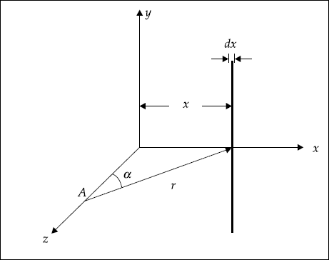
Fig. 2.7 A differential strip in an infinite surface charged sheet
or, |
dQ = ρs dS |
|
= ρs dx dy |
|
|
For a differential strip of width dx, we have
The field at a point, A on z-axis is given by
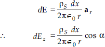
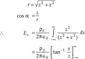
Here,
|
|
|
|
If the surface charge sheet lies in y-z plane, the field at a point on x-axis is
Similarly, if it is in x-z plane, the field at a point on y-axis is
In general, the field at a point on the axis normal to the plane of the sheet is given by
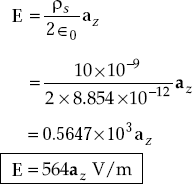
Problem 2.22 An infinite sheet in x-y plane extending from – ∞ to ∞ in both directions has a uniform charge density of 10 nC/m2. Find the electric field at z = 1.0 cm.
Solution ρs = 10 nC/m2
For a sheet of charge lying in x-y plane, the field at any point on z-axis is given by
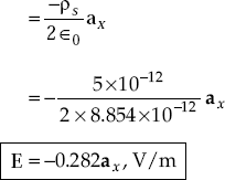
Problem 2.23 A sheet of charge lies in y-z plane at x = 0 and has uniform surface charge density of 5.0 PC/m2. Find the electric field at a point P (– 5, 0, 0) on x-axis.
Solution |
ρs = 5.0 PC/m2 |
|
= 5.0 × 10⁻¹² C/m2 |
E at P(–5, 0, 0)
Problem 2.24 A point charge, Q is at the centre of a neutral spherical conducting shell. Find the surface charge density at the inner surface and at the outer surface (Fig. 2.8).
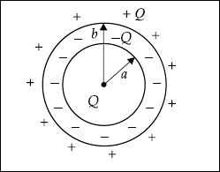
Fig. 2.8 Neutral spherical conducting shell
Solution The surface density at the inner surface is
The surface density at the outer surface is
Problem 2.25 A plane z = 1.0 m has a uniform charge density of ρs = 2.0 PC/m2. Find the electric field E above the plane.
Solution ρs = 2.0 × 10⁻¹² C/m2
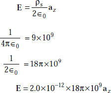
or, ![]()
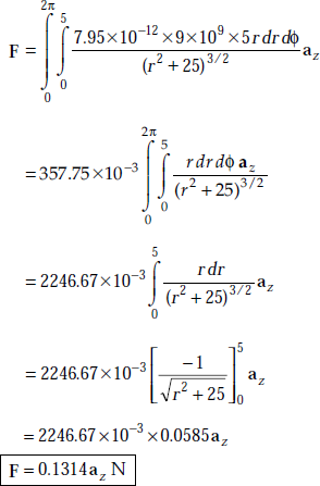
Problem 2.26 Determine the force on a point charge of 5 nC at (0, 0, 5) m due to uniformly distributed charge of 5 mC over a circular disc of radius r ≤ 1 m in z = 0 plane.
Solution Consider Fig. 2.9.
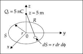
Fig. 2.9 Uniformly charged disc
The surface charge density, ρs is
From Fig. 2.9
The differential charge on dS is
Then the differential force due to differential charge is
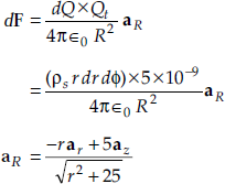
as
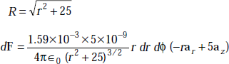
From Fig. 2.9, it is obvious that the radial components will be cancelled out due to symmetry.
The force on Qt is
2.12 FIELD DUE TO VOLUME CHARGE DENSITY, ρv (C/m3)
Volume charge density is defined as
|
|
|
|
Here, determination of field due to volume charge density simply involves the estimation of total charge, Q from ρv.
As
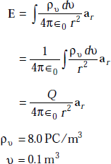
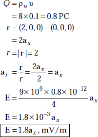
Problem 2.27 A sphere of volume 0.1 m3 has a charge density of 8.0 PC/m3. Find the electric field at a point (2, 0, 0) if the centre of the sphere is at (0, 0, 0).
Solution The field, E due to volume charge density is
Problem 2.28 Find the electric field at a point on the axis of a charged disc (Fig. 2.10).
Solution Consider a differential area shown by the dotted line.
The differential area = 2πr dr
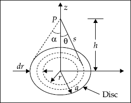
Fig. 2.10 Uniformly charged disc
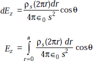
The field at P ![]()
The vertical component of E is
at |
r = 0, θ = 0 |
at |
r = a, θ = α |
Also |
r = h tan θ |
that is, |
dr = h sec2 θ dθ |
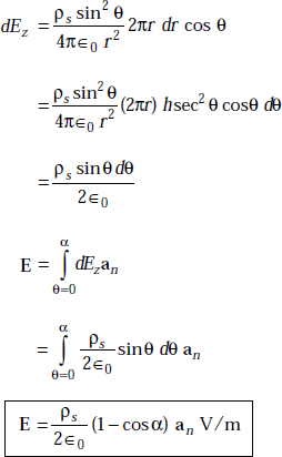
where ![]()
Problem 2.29 Determine the charge enclosed in a cylinder (Fig. 2.11) when the volume charge density is ρv = 1.0e–z (x2 + y2)–1/4 C/m3.
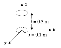
Fig. 2.11 Charge in a cylinder
Solution In cylindrical coordinates,
Hence the total charge
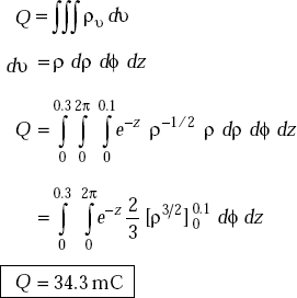
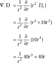
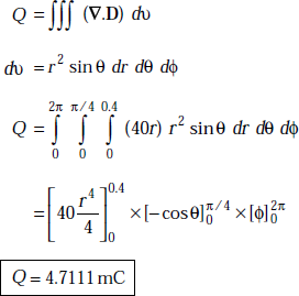
Problem 2.30 In a spherical region, the electric displacement is given by D = 10r2 ar mC/m2. Find the total charge enclosed by the volume specified by r = 40 cm, θ = π/4 and ϕ = 2π.
Solution The point form of Gauss’s law is
∇.D = ρv
and
But in the present problem, D is only a function of r, or, Dϕ = 0, Dθ = 0.
So,
2.13 POTENTIAL
A charge at rest produces potential at a specified point. It is a scalar quantity.
Potential at a point due to a fixed charge is defined as the work done in bringing one Coulomb of charge from infinity to the point against the force created by the fixed charge, that is, the potential is the work done per unit charge.
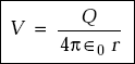
The potential, V at a point due to a fixed charge, Qf is given by
Simply ![]()
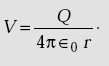
2.14 POTENTIAL AT A POINT
The potential at a point due to a point charge is given by
Proof Consider a fixed charge, Q and 1 C of charge at an infinite distance (Fig. 2.12). There exists a force on 1 C due to Q. If 1 C of charge is moved against the force of repulsion, some work has to be done.
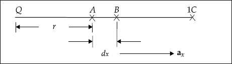
Fig. 2.12 Determination of potential
If 1 C is at point B which is at a distance of x from Q, then force on 1 C due to Q is
If 1 C is moved through a distance of dx in the opposite direction of ax, then the differential work done is
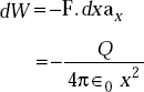
Total work done in moving 1 C from ∞ to r is
or,
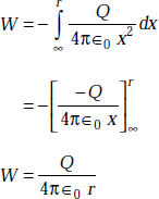
This work done is the potential. The potential at a distance of r from Q is
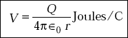
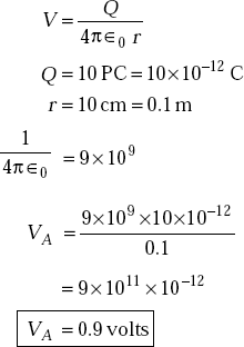
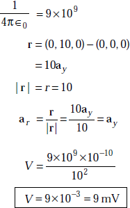
Problem 2.31 A charge of 10 PC is at rest in free space. Find the potential at a point, A 10 cm away from the charge.
Solution The potential at A is
Problem 2.32 The potential at a point A is 10 volts and at B it is 15 volts. If a charge, Q = 10μC is moved from A to B, what is the work required to be done?
Solution |
VA = 10 V |
|
VB = 15 V |
|
VBA = 15 – 10 = 5 volt |
|
|
|
Q = 10μC |
Work done |
= VBA × Q |
|
= 5 × 10μC |
|
W = 50μJ |
Problem 2.33 Two point charges Q1 = 2 nC and Q2 = 4 nC are located at (1, 1, 1) and (1, 0, 0) respectively. Determine the potential at P (1, 1, 0) due to the point charge.
Solution
Q1 = 2 nC
r1 = (1, 1, 1) = ax + ay + az
rp = (1, 1, 0) = ax + ay
rp – r1 = ax + ay – ax – ay – az
= –az
|rp – r1| = 1.0
The potential at P due to Q1 is
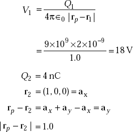
The potential at P due to Q2 is
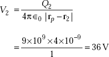
The total potential is V = V1 + V2 = 18 + 36
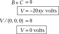
Problem 2.34 An electric field is given by E = 10yax + 10xay, V/m. Find the potential function, V. Assume V = 0 at the origin.
Solution We have
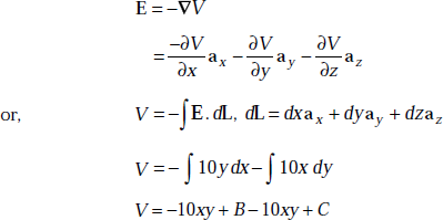
At x = 0 and y = 0, V = 0
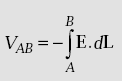
2.15 POTENTIAL DIFFERENCE
The potential difference between two points A and B is defined as the work done by an applied force in moving a unit positive charge from A to B in electric field.
The work done, 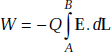
or, 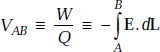
where Q = charge that is being moved from A to B.
Potential difference between A and B is also defined as the difference between the potentials at A and B.
Let VA be the potential at A. VB be the potential at B. Then
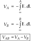
2.16 SALIENT FEATURES OF POTENTIAL DIFFERENCE
- Potential difference depends only on the initial and final points.
- It does not depend on the path between the points.
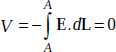
- It is zero around a closed path,
that is,
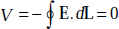
or,
- Negative value of VAB represents loss in potential energy in moving Q from A to B.
- Positive value of VAB represents gain in potential energy.
- VAB has the units of Joules/Coulombs or Volt.
- VAB depends on the distance between A and B.
- VAB is created by a fixed charge.
- If B is reference at ∞ from the fixed charge, VAB is the potential of A itself.
- The potential at ∞ is zero.
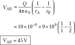
Problem 2.35 A point charge, Q = 10 nC is at the origin. Determine the potential difference at A (1, 0, 0) with respect to B (2, 0, 0).
Solution |
Q = 10 nC = 10 × 10–9 C |
|
rA = 1m |
|
rB = 2m |
The potential difference,
2.17 POTENTIAL GRADIENT
Potential gradient is defined as the gradient of potential, that is,
Potential gradient ≡ ∇V
where ∇ is vector differential operator and V is scalar potential.
2.18 SALIENT FEATURES OF POTENTIAL GRADIENT
- Potential gradient is a vector.
- It is always normal to equi-potential surfaces everywhere.
- It lies in the direction of maximum increase of potential.
- Negative potential gradient gives the electric field, that is,
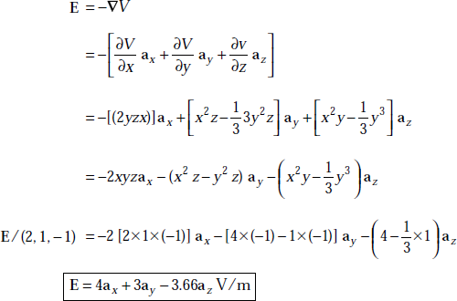
E = −∇V
- The electric field and potential gradient are in opposite directions.
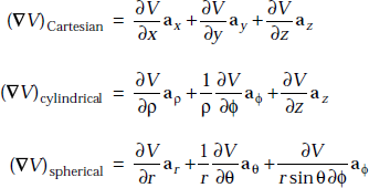
- The potential gradient in different coordinate systems is given by
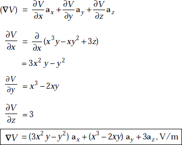
Problem 2.36 If the potential function, V is given by V = x3y – xy2 + 3z, find the potential gradient.
Solution V = x3y – xy2 + 3z
The potential gradient is given by
2.19 EQUIPOTENTIAL SURFACE
Equipotential surface is one on which the potential is the same on the entire surface.
Gradient of the potential and the equipotential surface are orthogonal to each other.
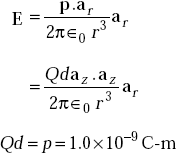
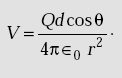
2.20 POTENTIAL DUE TO ELECTRIC DIPOLE
An electric dipole is defined as a pair of opposite polarity with identical magnitude and with a small distance between them.
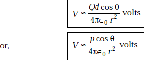
Potential due to a dipole
Here, |
Q = charge |
|
d= distance between two charges |
|
r = distance of the point from the centre of the pair of charges |
|
p = dipole moment = Qd (C-m) |
Electric field at a point due to a dipole
Proof Fig. 2.13 shows a dipole (A pair of charges)
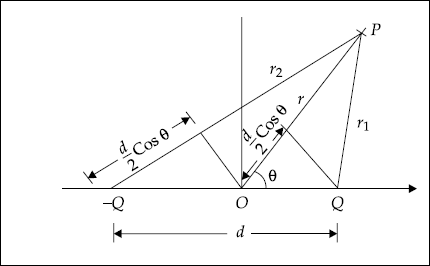
Fig. 2.13 An electric dipole
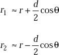
Let P be a point at which the potential and electric field are to be determined. Let r1 be the distance of P from (−) ve charge and be the distance of P from (+) ve charge and r2 be the distance from the centre of the dipole.
From Fig. 2.13, we have
Potential at P due to Q and –Q is
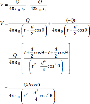
If
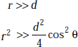
The expression for the potential becomes
where p = Qd = electric dipole moment.
If d cos θ is written as
Potential V becomes
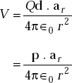
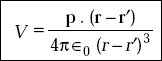
where p ≡ Qd is known as dipole moment. It is a vector and has the direction of d. Here d is the distance vector from –Q to Q. If the centre of the dipole is at r′ instead of at the origin, potential is given by
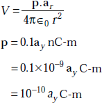
Problem 2.37 An electric dipole represented by 0.1ay nC-m is at the origin. Find the potential at a point P (0, 10, 0).
Solution We have
Problem 2.38 An electric dipole, 1.0ay nC-m is located at (0, 0, 0). Find the potential at ![]()
Solution The potential due to an electric dipole is given by
where
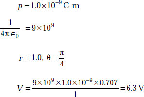
Hence ![]()
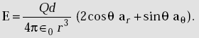
2.21 ELECTRIC FIELD DUE TO DIPOLE
In spherical coordinates, the gradient of the potential is given by
where ![]()
It is evident from the above expression that V is not a function of ϕ. Therefore,
E is only a function of r and θ.
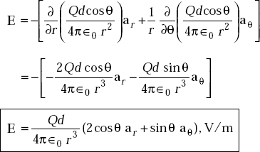
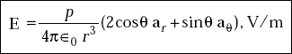
or in terms of electric dipole moment, E is expressed as
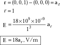
Problem 2.39 An electric dipole, 1.0az nC-m is at (0, 0, 0). Find the electric field at (0, 0, 1).
Solution We have
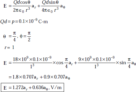
Problem 2.40 If an electric dipole located at the origin is represented by 0.1az nC-m, find E at ![]()
Solution We have
2.22 ELECTRIC FLUX
Electric flux is also known as Electric Displacement Flux.
Definition 1 Electric flux is defined as the displaced charge, that is,
Electric flux, Ψ ≡ Q, Coulomb.
Definition 2 Electric flux is defined as the surface integral of electric flux density, that is,
Electric flux, Ψ ≡ ![]()
2.23 SALIENT FEATURES OF ELECTRIC FLUX
- It is independent of the medium.
- The electric field creates a force on a charge and hence the charge moves along a certain path. This path is called the flux line.
- The force between two charges acts along a certain path. This path is also called the flux line.
- Magnitude of flux depends only on the charge from which it originates.
- The flux lines are equal to the charge in Coulombs.
- Flux line is only an imaginary line.
- Its direction is the same as that of the electric field.
- The flux lines from a point charge are shown in Fig. 2.14.
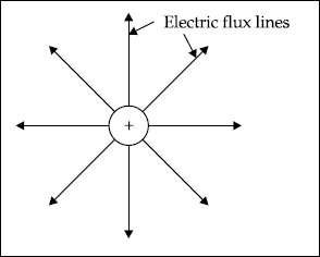
Fig. 2.14 Field from an isolated charge
- The flux lines between a (+)ve and a (–)ve point charges are shown in Fig. 2.15.
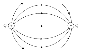
Fig. 2.15 The field in a system of equal but opposite charges
- It is a scalar quantity.
- The flux lines from a pair of (+)ve charges are shown in Fig. 2.16.
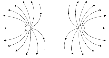
Fig. 2.16 Flux lines from two (+)ve charges
2.24 FARADAY’S EXPERIMENT TO DEFINE FLUX
Apparatus used One small metallic sphere, two hemispheres forming a full sphere larger than the small sphere, if held together over a dielectric material.
Procedure See the steps given below:
- Inner sphere is charged to Q Coulombs.
- Dielectric material is pasted radially over the sphere with uniform thickness.
- Two hemispheres are held together on the dielectric strip so that they form an outer sphere.
- Outer sphere is momentarily grounded to discharge its charge.
- The two hemispheres are removed with insulated tools without disturbing the induced charge.
- The charge on each sphere is measured.
- The total induced charge on the outer sphere is found to be negative.
- The magnitude of the induced charge is equal to that of the inner sphere.
- The displacement took place from inner to outer sphere through the dielectric material.
- This displacement is known as displacement flux.
- The displacement flux is also called electric flux.
- This flux is independent of the type of dielectric material.
- It is independent of the separation between inner and outer spheres.
- The final result of Faraday’s experiment is,
Electric flux, ψ = Q, Coulombs.
2.25 ELECTRIC FLUX DENSITY
This is also known as Displacement Electric Flux Density.
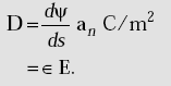
Definition 1 Electric flux density, D is defined as
where ψ is the electric flux crossing the differential area, dS. The direction of dS is always outward, normal to dS, that is, dS = dS an.
Definition 2 Electric flux density, D is also defined as
where |
∈0 = permittivity of free space, F/m |
|
E = electric field strength, V/m |
2.26 SALIENT FEATURES OF ELECTRIC FLUX DENSITY, D
- The unit of electric flux density is C/m2.
- It is a vector.
- It is inversely proportional to r2, r being the radius of the sphere.
- In free space, D is in the direction of E.
- D in a Gaussian surface is determined from Gauss’s law.
- D is independent of the medium.
- D is given by

- D in a general medium is given by
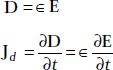
D = ∈ E
- D in a dielectric medium is given by
D = ∈0 E + P
P = polarisation of medium
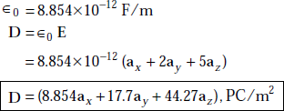
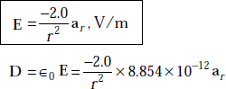
Problem 2.41 If an electric field in free space is given by
E = ax + 2ay + 5az V/m.
find the electric flux density.
Solution Electric field, E = ax + 2a y + 5a z
Problem 2.42 A point charge, Q = 10 nC is at the origin in free space. Find the electric field at P (1, 0, 1). Also find the electric flux density at P.
Solution
Q = 10 nC = 10 × 10−9 C
P = (1, 0, 1)
r = (1, 0, 1) − (0, 0, 0)
= ax + az
Electric field,
The electric flux density,
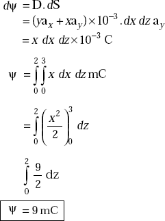
Problem 2.43 What is the electric flux, ψ that passes the surface shown in Fig. 2.17, if the displacement flux density is D = yax + xay mC/m2.
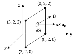
Fig. 2.17 Electric flux
Solution Electric flux density is given by
D = ya x + xa y (mC/m2)
The differential area, dS is given by
dS = dx dz a y
The differential flux, dψ passing through dS is
2.27 GAUSS’S LAW AND APPLICATIONS
Generalised Faraday’s law is Gauss’s law.
Gauss’s law It states that the net flux passing through any closed surface is equal to the charge enclosed by that surface, that is,
This is known as Gauss’s law in integral form. Gauss’s law is applicable only on Gaussian surfaces.
Proof Consider a spherical surface which encloses a charge Q at its centre (Fig. 2.18).
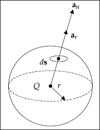
Fig. 2.18 Spherical surface enclosing a charge, Q
The differential area, ds is on the surface of the sphere whose direction is an. Let r be the radius of the sphere.
The electric field, E at the spherical surface is given by
|
|
|
|
Taking dot product with ds on both sides, we get
For the spherical surface under consideration, ar and an are in the same direction.
Taking surface integral on both sides, we get
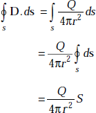
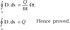
But S = 4πr2 for a sphere. So,
2.28 PROOF OF GAUSS’S LAW (ON ARBITRARY SURFACE)
Consider an arbitrary surface of Fig. 2.19.
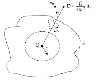
Fig. 2.19 Arbitrary surface to prove Gauss’s law
Consider a sphere of radius one metre within the surface, S which encloses a charge, Q at its centre.
Electric flux density, D at ds on the arbitrary surface is
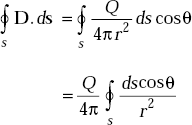
Taking dot product with ds on both sides
Here, if ar and an make an angle of θ, then
Now taking surface integral on both sides,
On the right hand side, the integrand consists of ![]() The numerator dscosθ represents the projection of area ds on the spherical surface whose radius is r. Hence
The numerator dscosθ represents the projection of area ds on the spherical surface whose radius is r. Hence ![]() will be the projection of ds on the spherical surface of radius equal to unity. This is the solid angle subtended by an area ds at the location of the point charge. Therefore,
will be the projection of ds on the spherical surface of radius equal to unity. This is the solid angle subtended by an area ds at the location of the point charge. Therefore,  is the total solid angle subtended by s at the point charge. It is the sum of the projections of all ds on the spherical surface of radius unity and centered at Q. This is equal to the area of the spherical surface of unity radius. Hence
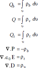
2.29 GAUSS’S LAW IN POINT FORM
Gauss’s law in point form states that the divergence of electric flux density is equal to the volume charge density, that is,
Proof Consider a differential parallelepiped as shown in Fig. 2.20.
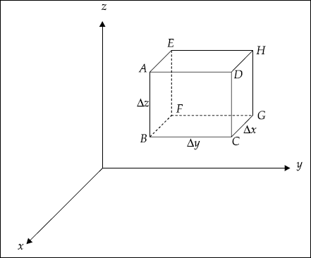
Fig. 2.20 Differential parallelepiped
Assumptions
- The differential parallelepiped has the dimensions ∆x, ∆y and ∆z.
- The point, P is in the centre of the element.
- The flux density D at the centre is given by
D = Dc = Dcx ax + Dcy ay + Dcz az
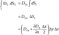
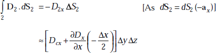
The integral form of Gauss’s law is
where
Face 1 represents the face ABCD
Face 2 represents the face EFGH
Face 3 represents the face ABFE
Face 4 represents the face DCGH
Face 5 represents the face ADHE
Face 6 represents the face BCGF
D1, D2, D 3, D4, D5 and D6 are the flux densities on the faces 1, 2, 3, 4, 5 and 6 respectively.
dS1, dS2, dS3, dS4, dS5 and dS6 are differential areas of the faces 1, 2, 3, 4, 5 and 6, respectively.
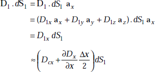
As the flux density at the centre is known, it is found on each face of the parallelepiped by considering the first two terms of Taylor’s theorem.
Taylor’s theorem states that if f (x) has continuous derivatives in the neighbourhood of a point x = a, then
If (x − a) is very small, we have
Accordingly, we can simplify D1, D2, D3, D4, D5 and D6
Similarly
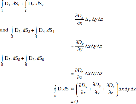
If
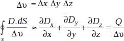
This becomes exact if Δv → 0.
But

2.30 DIVERGENCE OF A VECTOR, ELECTRIC FLUX DENSITY
The divergence of electric flux density is defined as
This means that the divergence of flux density is the outflow of electric flux from a closed surface per unit volume as the volume shrinks to zero.
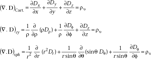
The point form of Gauss’s law in different coordinate systems is
2.31 APPLICATIONS OF GAUSS’S LAW
- It is useful to find flux, ψ or flux density, D from the knowledge of enclosed charge and surface.
- It is useful to find the electric field from the knowledge of enclosed charge and surface.
- It is useful to find the enclosed charge from the knowledge of either D or E.
2.32 LIMITATIONS OF GAUSS’S LAW
- It cannot be applied on Non-Gaussian surfaces.
- It can be applied only if the surface encloses the volume completely.
2.33 SALIENT FEATURES OF GAUSS’S LAW
- It relates volume integral to surface integral.
- It is applicable only if the surface completely encloses the volume.
- It does not specify any particular shape for the closed surface.
- It does not require knowledge of the distance from the points on the surface.
- It cannot be applied if the charges are outside the surface.
- It is useful to find D or E from the knowledge of the charge enclosed and the surface.
- It is applicable only on Gaussian surfaces.
- It is useful to find the outward flow of flux from a closed surface from the enclosed charge.
Problem 2.44 If electric flux density, D is given by,
D = [(2y2 + z) ax + 4xy ay + xaz)] μC/m2
find the volume charge density at (0, 0, 0) and (−1, 0, 4).
Solution
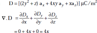
But ρv = volume charge density = ∇.D
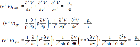
2.34 POISSON’S AND LAPLACE’S EQUATIONS
Poisson’s equation ![]()
Laplace’s equation ∇2 V = 0
Proof The point form of Gauss’s law is
|
∇.D = ρv |
But |
D = ∈ E |
and |
E = −∇V |
|
∇.D = ∇.∈ E = ∇.∈ (−∇V) = ρv |
or, ![]()
[as ∇ . ∇ = ∇2]
where ∇2 is a scalar operator ![]() and is called Laplace’s operator.
and is called Laplace’s operator.
In the regions where ρv = 0, Poisson’s equation becomes
Laplace’s equation in one dimensional form is given by
Its solution is in the form of
Laplace’s equation in two dimensional form is given by
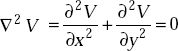
Its solution is given by
where r is the radius of a circle about a point (x, y).
Laplace’s equation in three dimensional form is given by
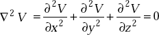
The value of V at point p is the average value of V over a spherical surface of radius r centered at p and it is given by
Poisson’s equation in different coordinates
2.35 APPLICATIONS OF POISSON’S AND LAPLACE’S EQUATIONS
- They are useful in determining surface charge densities and electric field in the regions of interest.
- They can be used to find the capacitance of different structures by appropriate application of boundary conditions.
2.36 UNIQUENESS THEOREM
It states that either Poisson’s or Laplace’s equation has only one solution.
Proof Assume that V1 and V2 are the solutions of Laplace’s equation and V1b and V2b are the potentials on the boundaries. By hypothesis,
|
∇2 V1 = 0 |
and |
∇2 V2 = 0 |
|
∇2 (V1 − V2) = 0 |
As V1b and V2b are the values on the boundary we have
|
V1b = V2b = Vb |
or, |
V1b − V2b = 0 |
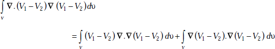
Consider a vector identity, namely
where ψ is a scalar and A is a vector quantity.
This is valid for any scalar, ψ and any vector, A.
In the present case, let ψ = V1 – V2, A = ∇ (V1 – V2). Then, the above identities become
Take volume integral on both sides
Applying divergence theorem to the left hand side, volume integral is replaced by surface integral,
that is,
But on the boundary, this becomes
Right hand side is zero because V1b = V2b. By hypothesis
So the remaining integral is
This is possible if
- Integrand is zero.
- Integrand is positive in some region and negative in some other region.
The second condition cannot be true as it is a square term.
So the integrand is zero,
that is, [∇(V1 − ∇2)]2 = 0 or ∇ (V1 − V2) = 0
If the gradient of a scalar is zero everywhere, then (V1 – V2) cannot change with any coordinate. Hence (V1 – V2) = constant.
The constant is easily evaluated by considering a point on the boundary. Here V1 – V2 = V1b – V2b = 0,
that is, ![]() Hence proved.
Hence proved.
Problem 2.45 Consider concentric spherical shells in free space in which V = 0 volts at r = 10 cm and V = 10 volts at r = 20 cm. Find E and D.
Solution Here V is a function of only r and not θ, and ϕ. Then Laplace’s equation
Integrating twice, we get
The boundary conditions are
V = 0 V at r = 10 cm = 0.1 m and
V = 10 V at r = 20 cm = 0.2 m,
that is,
So, 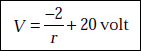
But ![]()
or,
or, 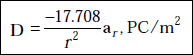
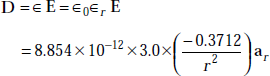
Problem 2.46 There exists a potential of V = –2.5 V on a conductor at 0.02 m and V = 15.0 V at r = 0.35 m. A dielectric material whose ∈r = 3.0 exists between the conductors. Determine the surface charge densities on the conductors.
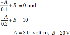
Solution As V is a function of only r, Laplace’s equation is given by
Integrating twice, we get
A and B can be found by the use of boundary conditions,
that is,
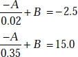
Solving, we get
A = 37.12 × 10⁻² , V-m
B = 16.06
and ![]()
But
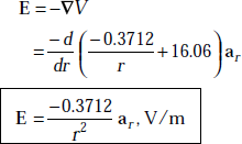
and
or, 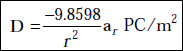
On the conductor surfaces,
|
Dn = ρs = surfacedensity |
At |
r = 0.02 m |
|
ρs = −2.4649 × 10⁻⁸ C/m2 |
or, ![]()
At
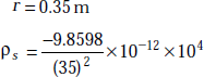
or, ![]()
Problem 2.47 In what manner does permittivity vary to satisfy Laplace’s equation in a non-homogeneous, charge-free space?
Solution For charge-free space,
|
ρv = 0 |
|
|
∇.D = 0 |
|
|
∇.∈ E = 0 |
[as D = ∈ E] |
|
∇.(−∈ ∇V) = 0 |
[as E = − ∇V] |
|
∇.(∈ ∇V) = 0 |
|
If ∈ varies spatially, then
|
∇.(∈∇V) = ∇V.∇∈ + ∇2 V = 0 |
As |
∇2 V = 0 |
|
(∇V).(∇∈) = 0 |
This is true only when ∇V and ∇∈ are perpendicular to each other. Hence permittivity should vary so that its gradient is perpendicular to the electric field.
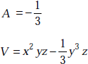
Problem 2.48 If a potential V = x2 yz + Ay3 z, (a) find A so that Laplace’s equation is satisfied (b) with the value of A, determine electric field at (2, 1, −1).
Solution (a) Laplace’s equation is
or, ![]()
As V = x2 yz + Ay3 z
The above equation becomes
So, ![]()
(b) With
But
2.37 BOUNDARY CONDITIONS ON E AND D
- The tangential component of E is continuous across any boundary, that is,
 or
orThe tangential component of E in medium 1 is the same as that of E in medium 2 at any boundary.
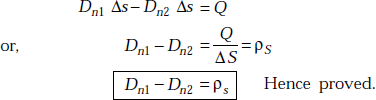
- The normal component of D is continuous across any boundary except at the surface of the conductor. In general,
ρs = surface charge density, (C/m2). For any point other than the conductor boundary, Dn1 = Dn2.
2.38 PROOF OF BOUNDARY CONDITIONS
Consider the rectangular loop on the boundary of two media (Fig. 2.21).
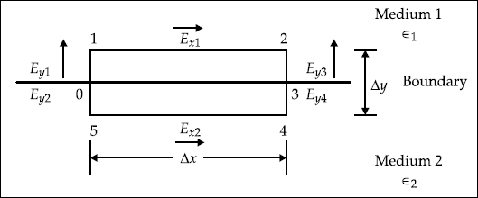
Fig. 2.21 Rectangular loop on boundary
It is well known that electric field is conservative and hence the line integral of E .dL is zero around a closed path,
that is, ![]()
From the figure shown above, LHS is written as
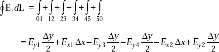
As Δy → 0, we get
Thus, Ex1 = Ex2
It is obvious that Ex1 and Ex2 are the tangential components of E in medium 1 and 2 respectively.
So, Etan1 = Etan2
Now consider a cylinder across the media 1 and 2 (Fig. 2.22).
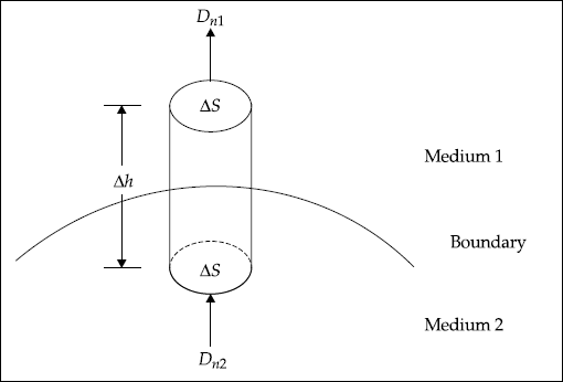
Fig. 2.22 Cylindrical surfaces on boundary
According to Gauss’s law,
Applying this to the cylindrical surface on the boundary spreading over medium 1 and medium 2, we get Δh → 0
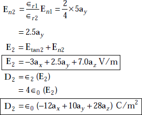
Problem 2.49 The region y < 0 contains a dielectric material for which ∈r1 = 2.0 and the region y > 0 contains a dielectric material for which ∈r2 = 4.0. If E1 = –3.0ax + 5.0ay + 7.0az V/m, find the electric field, E2 and D2 in medium 2.
Solution As y < 0 belongs to medium 1 and y > 0 belongs to medium 2
Etan1 = −3.0ax + 7.0az V/m
En1 = 5.0ay V/m
∈r1 = 2
∈r2 = 4
The boundary condition on tangential component of E is
Etan1 = Etan2
Etan2 = −3.0ax + 7.0az V/m
and
Problem 2.50 An electric field in medium 1 of ∈r1 = 7 passes into a medium 2 of ∈r2 = 2. When the field, E makes an angle of 60° as shown in Fig. 2.23 with the axis normal to the boundary line, find the angle made by the field with the normal in medium 2.
Solution From Fig. 2.23
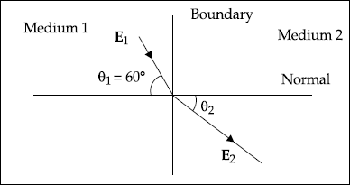
Fig. 2.23
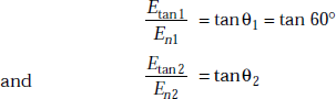
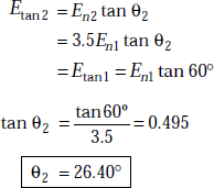
According to the boundary conditions,
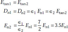
and
2.39 CONDUCTORS IN ELECTRIC FIELD
Conductors
Definition 1 Conductors are materials which have very low resistance. Examples: Copper, Silver and Aluminium.
Definition 2 Conductors are materials for which no forbidden gap exists between valance band and conduction band.
Definition 3 A material is defined as a conductor ![]()
Conductors have a variety of applications in all fields of life.
2.40 PROPERTIES OF CONDUCTORS
- Charge density is zero within a conductor.
- The surface charge density resides on the exterior surface of a conductor.
- In static conductors, current flow is zero.
- Electric field is zero within a conductor.
- Conductivity is very large.
- Resistivity is small.
- Magnetic field is zero inside a conductor.
- Good conductors reflect electric and magnetic fields completely.
- A conductor consists of a large number of free electrons which constitute conduction current with the application of an electric field.
- A conductor is an equipotential body.
- The potential is same everywhere in the conductor.
- E = –∇V = 0 in a conductor.
- In a perfect conductor, conductivity is infinity.
- When an external field is applied to a conductor, the positive charges move in the direction E and the negative charges move in the opposite direction. This happens very quickly.
- Free charges are confined to the surface of the conductor and hence surface charge density, Js is induced. These charges create internal induced electric field. This field cancels the external field.
It is interesting to note that copper and silver are not super conductors but aluminium is a superconductor for temperature below 1.14 K.
2.41 ELECTRIC CURRENT
The current through a given medium is defined as charge passing through the medium per unit time. It is a scalar, that is,
Current is of three types.
- Convection current
- Conduction current
- Displacement current
- Convection current It is defined as the current produced by a beam of electrons flowing through an insulating medium. This does not obey Ohm’s law. For example, current through a vacuum, liquid and so on is convection current.
- Conduction current It is defined as the current produced due to flow of electrons in a conductor. This obeys Ohm’s law. For example, current in a conductor like copper is conduction current.
- Displacement current It is defined as the current which flows as a result of time-varying electric field in a dielectric material. For example, current through a capacitor when a time-varying voltage is applied is displacement current.
2.42 CURRENT DENSITIES
In electromagnetic field theory, it is of interest to describe the events at a point instead of in a large region. This is the reason why current densities are considered. Current densities are vector quantities.
Current Density is defined as the current at a given point through a unit normal area at that point. It is a vector and it has the unit of Ampere/ m2. It is represented by J.
Current densities are of three types:
- Convection current density
- Conduction current density
- Displacement current density
- Convection current density (A/m2) It is defined as the convection current at a given point through a unit normal area at that point, that is,
Convection current density

where
dI = differential convection current
dS = differential area
= dSan
an = outward unit normal to dS
As convection current density is confined to specific media, it is not of much interest in this book.
- Conduction current density, Jc (A/m2) It is defined as the conduction current at a given point through a unit normal area at that point,
that is,
Jc ≡ σE
and
Conduction current density exists in the case of conductors when an electric field is applied.
- Displacement current density, Jd (A/m2) It is defined as the rate of displacement electric flux density with time, that is,

If Id is the displacement current in a dielectric due to applied electric field, displacement current density is defined as

As
In fact, displacement current density exists due to displacement of bound charges in a dielectric by the applied electric field.
2.43 EQUATION OF CONTINUITY
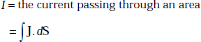
Equation of continuity in integral form is ![]()
I = outward flow of current (A)
J = conduction current density (A/m2)
where ![]()
Proof If Qi is the charge inside a closed surface, the rate of decrease of charge due to the outward flow of current is given by 
From the principle of conservation of charge, we have
From divergence theorem, we have
So,
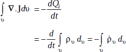
Two volume integrals are equal if the integrands are equal. So,
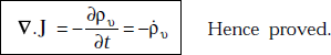
In the above equation the derivative became a partial derivative as the surface is kept constant.
2.44 RELAXATION TIME (Tr)
It is also called rearrangement time.
Relaxation time is defined as the time taken by a charge placed in a material to reach 36.8 per cent of its initial value. It is given by
where ∈ = permittivity (F/m), σ = conductivity (mho/m).
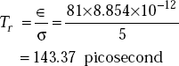
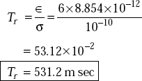
Problem 2.51 Find the relaxation time of sea water whose ∈r = 81 and σ = 5 mho/m.
Solution Relaxation time of sea water
Problem 2.52 Find the relaxation time of porcelain whose σ = 10–10 mho/m, ∈r = 6.
Solution Relaxation time of porcelain
2.45 RELATION BETWEEN CURRENT DENSITY AND VOLUME CHARGE DENSITY
J = conduction current density, A/m2
V = velocity of the charge (m/s)
Proof We know that ![]()
Consider an element charge (Fig. 2.24)
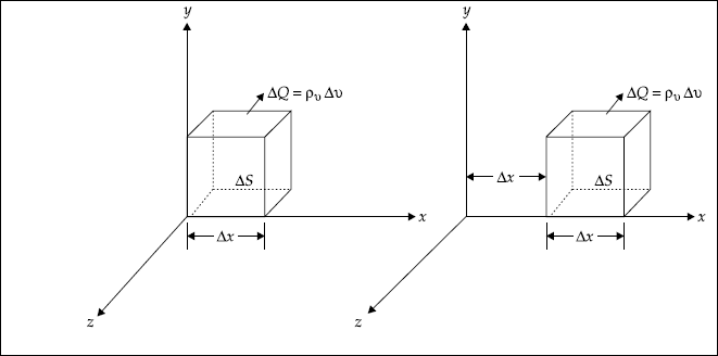
Fig. 2.24 Volume charge in motion
Assume that the charge element is oriented parallel to the coordinate axes. Let there be only an x-component of velocity. It moves a distance of Δx in a time Δt as in the figure. Therefore,
The resultant current is
where Vx = x -component of velocity of the charge.
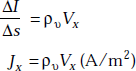
Similarly, if the charge moves in y and z-directions, we get
|
Jy = ρv Vy |
|
Jz = ρv Vz |
|
J = ρv (Vx ax + Vy ay + Vz az) |
As |
V = Vx ax + Vy ay + Vz az |
|
|
Problem 2.53 If the current density, ![]() find the current passing through a sphere radius of 1.0 m.
find the current passing through a sphere radius of 1.0 m.
Solution ![]()
where
where
that is,
Problem 2.54 Find the electric flux density in free space if the electric field, E = 6ax – 2ay + 3az , V/m.
Solution Electric field in free space,
E = 6ax − 2ay + 3az , V/m
∈0 = 8.854 × 10⁻¹²
The electric flux density,
2.46 DIELECTRIC MATERIALS IN ELECTRIC FIELD
Definition 1 An ideal dielectric material is one which does not contain free electrons.
Definition 2 An ideal dielectric material is one in which the charges are well bounded and cannot be set in motion easily.
Definition 3 An ideal dielectric material is one for which there exists a large forbidden gap between valance band and conduction band.
Definition 4 A material is defined as dielectric material if ![]()
Definition 5 A material is defined as dielectric material if it does not conduct electric current and opposes the flow of current.
2.47 PROPERTIES OF DIELECTRIC MATERIALS
- Conductivity is zero.
- Volume charge density, ρν = 0.
- Electric and magnetic fields exist in a dielectric material.
- Resistivity is ∞.
- Electric and magnetic fields penetrate the dielectric material freely.
- There exists no free electrons.
Dielectrics in Electric Field
An atom of a dielectric consists of a nucleus and a bunch of electrons. Similarly, a molecule of a dielectric consists of nuclei and a set of electron bunches. The charge of the nucleus is positive and the charge of the electron bunch is negative. The atoms and molecules are electrically neutral as they contain an equal number of negative and positive charges.
Dielectrics are classified into polar and non-polar type of materials.
Polar type of dielectrics
The centres of positive and negative charges of a molecule of polar type of dielectric material are separated by a small distance. Each pair acts as a dipole and there exists a dipole moment. However, such pairs are randomly distributed in a dielectric material. Hence the overall dipole moment is zero.
If such a material is kept in an electric field, all the positive charges move in the direction of the electric field and all the negative charges move in the opposite direction. As a result, dipole moment is induced by the electric field. Under these conditions, the material is said to be under a state of polarisation.
A polar type of molecule is shown in Fig. 2.25.
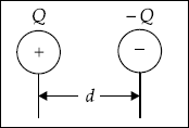
Fig. 2.25 Polar type of molecule
Examples of polar dielectrics are water, hydrochloric acid, sulphur dioxide and others.
Non-polar type of dielectrics
The centres of positive and negative charges of a molecule of non-polar type of dielectric material coincide as in Fig. 2.26, that is, there is no separation between them and hence dipole moment is zero.
However, when such a material is placed in an electric field, the centres of positive and negative charges are displaced and there exists a distance between them, that is, dipole moment is induced. Under these conditions, the material is said to be under a state of polarisation.
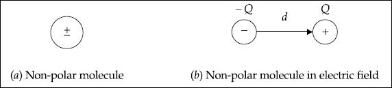
Fig. 2.26
Examples of non-polar dielectrics are oxygen, hydrogen, nitrogen and so on.
The important conclusion is that dielectric materials are not polarised in the absence of electric field and they are polarised in the presence of an electric field. As a result, the electric flux density is greater than that in free space conditions with the same field intensity. The intensity of polarisation is described in terms of dipole moment and polarisation.
2.48 DIPOLE MOMENT, p
It is defined as the product of charge and distance between the centres of (+)ve and (–)ve charges of a molecule,
that is, |
p ≡ Qd, (C-m) |
where |
p = dipolemoment |
|
Q = charge magnitude |
|
d = distance vector from(−)ve to(+)ve charges of the dipole |
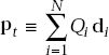
If there are N dipoles in a dielectric material of volume Δν, the total dipole moment with the application of electric field is
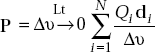
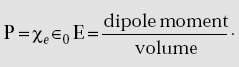
2.49 POLARISATION, P
Polarisation is defined as the dipole moment per unit volume of the dielectric,
that is,
In some dielectrics, the polarisation, P is defined as
|
P ≡ χe ∈0 E |
where |
χe = electric susceptibility of the dielectric |
The charges are bound in a dielectric and the total positive bound charge on a surface, S enclosing the dielectric is given by
On the other hand, the charge that remains inside the surface, S is –Qb and it is given by
If there is some free charge in the dielectric, the free charge volume charge density is ρν. If ρb is the bound volume charge density, then the total volume charge density is given by
ρt = ρv + ρb
= ∇.∈ E
or,
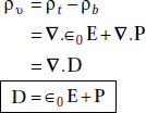
As P ≡ χe ∈0 E, we have
D = ∈0 E + χe ∈0 E
= ∈0 E (1 + χe)
D = ∈0 ∈r E = ∈ E
where ![]()
or, ![]()
In summary, we have
Problem 2.55 A pair of negative and positive charges of 10 μC each are separated by a distance of 0.1 m along the x-axis. Find the dipole moment.
Solution |
Q1 = −10μC |
|
Q2 = 10μC |
|
d = 0.1ax |
|
Q = 10μC |
The dipole moment is
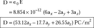
Problem 2.56 If a dielectric material of ∈r = 4.0 is kept in an electric field E = 3.0a x + 2.0a y + a z, V/m, find the polarisation.
Solution
∈r = 4.0
E = 3.0ax + 2.0ay + az
Polarisation in the dielectric,
P = χe ∈0 E
χe = ∈r −1
= 4 − 1 = 3
P = 3 × 8.854 × 10−12 × (3ax + 2ay + az)
= (79.68ax + 53.12ay + 26.56az) PC/m2
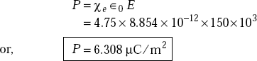
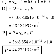
Problem 2.57 What are the magnitudes of electric flux densities and polarisation for a dielectric material in which E = 150 kV/m? Electric susceptibility of the dielectric material is 4.75.
Solution We have
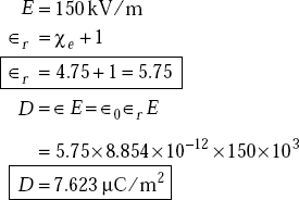
Polarisation is
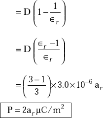
Problem 2.58 Find the polarisation, P in a homogeneous and isotropic dielectric material whose ∈r = 3.0 when D = 3.0ar μC/m2.
Solution Polarisation,
|
|
P = χe ∈0 E |
|
and |
D = ∈0 ∈r E, χe = ∈r − 1 |
|
|
D = ∈0 E + P |
|
or, |
P = D−∈0 E |
Problem 2.59 If the polarisation P = 3a x nC/m2 in a homogeneous and isotropic dielectric material whose χe = 4.5, find E in the material.
Solution We have
P = 3ax nC/m2
= χe ∈0 E
or,
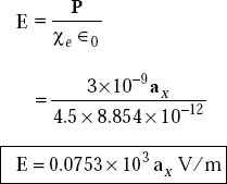
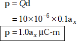
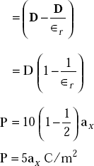
Problem 2.60 A dielectric slab (∈r = 2) is placed under the influence of electric flux density = 10ax C/m2 . The slab has a volume of 0.1 cm3 . Determine the polarisation in the slab and total dipole moment.
Solution The electric flux density,
|
D = ∈0 E + P |
or, |
P = D −∈0 E |
|
|
Dipole moment, |
p = polarisation × volume |
Slab volume |
= 0.1 cm3 = 0.1 × (10−2)3 = 10−7 m3 |
|
|
Problem 2.61 What are the magnitudes of P and D for a dielectric material in which E = 1.0 V/m and χ e = 5.0?
Solution
2.50 CAPACITANCE OF DIFFERENT CONFIGURATIONS
Any two conducting bodies separated by free space or a dielectric material exhibit a capacitance between them.
Capacitance is defined as the ratio of the absolute value of charge to the absolute value of the voltage difference,
that is, ![]()
Capacitance depends only on the geometry of the system and properties of the dielectrics involved. It does not depend on Q and V.
The capacitance of a capacitor is the ability to store electric charge. It opposes sudden changes in voltage. Its reactance is ![]() ohms. Here f is the frequency and C is capacitance in Farads.
ohms. Here f is the frequency and C is capacitance in Farads.
Capacitance of a parallel plate capacitor It is given by
where |
= permittivity of the dielectric between the conductors (F/m) |
|
A = area of the conductor |
|
d = distance between the conductors |
Proof Consider Fig. 2.27.
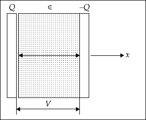
Fig. 2.27 Parallel plate capacitor
Let Q be the absolute charge on one of the plates, V be the potential difference between them, d be the distance between the plates, A be the area of the plate and ∈ be the permittivity of the medium between the plates.
Then the electric flux density is
Potential difference between the plates is
Capacitance of parallel plate capacitor of n dielectric slabs
It is given by 
where |
di = width of the ith slab |
|
∈i = permittivity of the ith slab |
Proof Let ∈1, ∈2, ∈3,…, ∈n be the permittivity of dielectric materials between the plates; d1, d2, d3,…, dn respectively be their thickness. (Fig. 2.28).
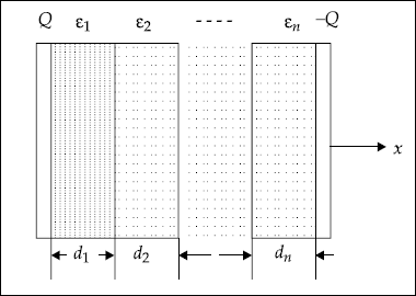
Fig. 2.28 Parallel plate capacitor with multi dielectrics
The potential difference across the capacitor is
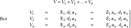
If Q is the charge on the plates, then the electric flux density, D is
Then
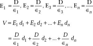
or,
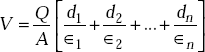
Hence 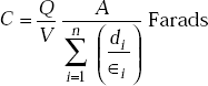 Hence proved.
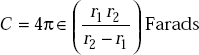
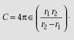
Capacitance between two concentric spheres
It is given by
where |
r1 = radius of the inner sphere |
|
r2 = radius of the outer sphere |
Proof Refer Fig. 2.29.
Fig. 2.29 Concentric spheres
The radial electric field is given
Potential difference between the two spheres is given by
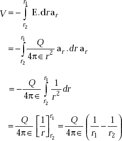
If r2 is ∞, the structure will result in an isolated sphere.
The capacitance of an isolated sphere of radius r,1 = r is
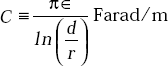
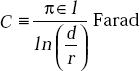
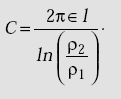
Capacitance of a coaxial cable
It is given by
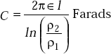
where |
l = length of the cable |
|
ρ1, ρ2 = radius of inner and outer conductors |
|
∈ = permittivity of the dielectric between the conductors |
Proof Refer Fig. 2.30.
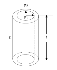
Fig. 2.30 Coaxial cable
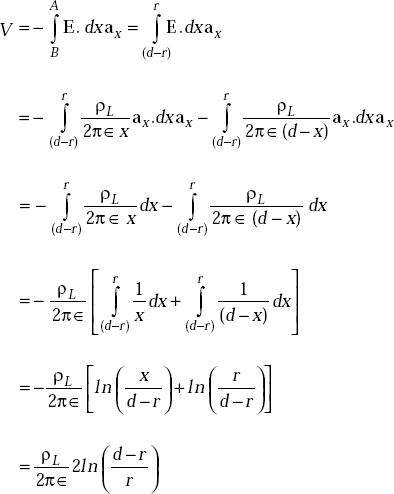
Let ρ1, and ρ2 be the radii of the inner and outer conductors of the coaxial cable. Let ρL be the line charge density on the inner conductor and -ρ L be that on the outer conductor. Then the electric field in the radial direction is
The potential difference between the cylinders is
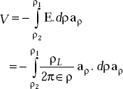
or,
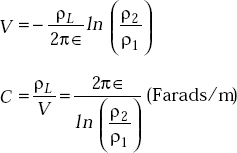
The capacitance of a cable of length l metres is
 Hence proved.
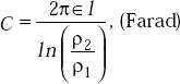
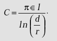
Capacitance of parallel wires
It is given by
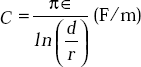
where |
d = distance between the wires |
|
r = radius of each conducting wire |
Proof Refer Fig. 2.31.
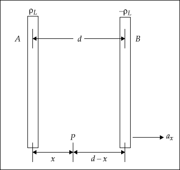
Fig. 2.31 Parallel wires like power transmission lines
Let ρL and -ρL be the line charge densities of the lines A and B respectively. Let d be the distance between the wires and r be the radius of each wire.
Electric field between the wires at the point P due to ρL is
Electric field at P due to -ρL is
The potential difference, V
that is,
In all practical cases, d >> r. As a result ![]()
So,
The capacitance,
or capacitance of a pair of wires of length l metres is, therefore, given by
Problem 2.62 Find the capacitance of an isolated sphere of radius 1 cm.
Solution The expression for the capacitance of an isolated sphere is
|
C = 4π ∈0 r |
Here |
r = 1 cm = 0.01m |
|
C = 4π ∈0 × 0.01 m |
Problem 2.63 A parallel plate capacitor has conducting plates of area equal to 0.04 m2. The plates are separated by a dielectric material whose ∈r = 2 with the plate separation of 1 cm. Find (a) its capacitance value (b) the charge on the plates when a potential difference of 10 V is applied (c) the energy stored.
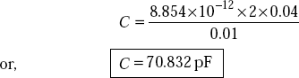
Solution (a) The capacitance of parallel plate capacitor, C
where |
∈ = ∈0∈r = 2 ∈0 |
|
A = 0.04 m2 |
|
d = 1 cm = 0.01 m |
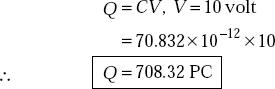
(b) We have
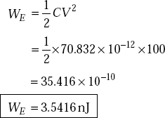
(c) Energy stored
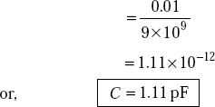
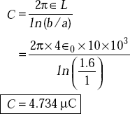
Problem 2.64 Find the capacitance for a 10 km long coaxial cable shown in Fig. 2.32.
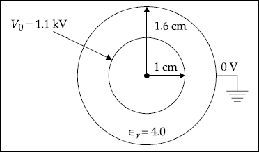
Fig. 2.32 Coaxial cable
Solution For the coaxial cable shown, the inner radius, a = 1 cm, and outer radius, b = 1.6 cm.
The capacitance of the cable is,
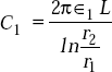
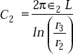
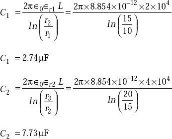
Problem 2.65 The cable shown in Fig. 2.33 is 10 km long. If r1 = 10 mm, r2 = 15 mm, r3 = 20 mm, ∈r1 = 2.0, r2 = 4.0, find the capacitance of the cable.

Fig. 2.33 Coaxial cable
Solution The capacitance of the two inner conductors
The capacitance of the two outer conductors
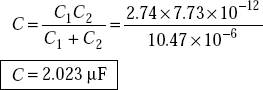
As these two are in series, the resultant capacitance, C
But
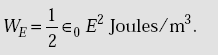
2.51 ENERGY STORED IN AN ELECTROSTATIC FIELD
Energy density in an electrostatic field is given by
When a positive charge is brought from a distance of infinity to a point in a field of another positive charge, work is done by an external source. Energy spent in doing so represents the potential energy.
If the external source is removed, the charge that is brought moves back, acquiring kinetic energy of its own and it is capable of doing some work.
If V is the potential at a point due to some fixed charge,
Work done = potential energy
that is, WE = QV
where Q is the charge brought by an external source,
V is the potential at the point due to a fixed charge.
Let us consider two charges Q1 and Q2 separated by a distance of infinity. If Q1 is fixed, work done on bringing Q2 towards Q1 is given by
where ![]()
Similarly, consider another charge, Q3 which is at infinity from Q1 and Q2. Now work done in bringing Q3 towards Q1 and Q2
This is because there exists force due to Q1 and Q2 after Q2 is brought toQ1.
In the above equation, ![]() are the potentials at Q3 due to Q1 and Q2 respectively. Therefore, total work done in bringing Q2 and Q3 is
are the potentials at Q3 due to Q1 and Q2 respectively. Therefore, total work done in bringing Q2 and Q3 is
In a similar fashion, consider n charges. Then we have

that is, 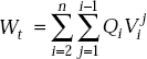
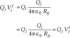
where ![]() is the potential of Qj at the location of Qi. Note that
is the potential of Qj at the location of Qi. Note that
Wt may be written as
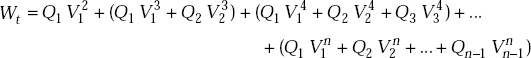
Adding the above two equations and simplifying, we get
|
= Q1 × (potential at Q1 due to all other charges) + Q2 × (potential at Q2 due to all other charges) + Qn × (potential at Qn due to all other charges) |
|
= Q1 V1 + Q2 V2 + …Qn Vn |
or,
This equation represents the potential energy stored in a system of n point charges.
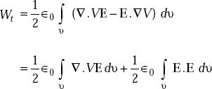
|
|
|
|
But |
∇.D = ρυ or ∇.E = ρυ/∈0 |
|
|
From standard vector identity,
this becomes
Applying divergence theorem, first term on the right hand side can be written as
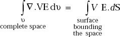
However, viewing from a surface bounding complete space, the charge distribution of finite volume appears as a point charge, say Q. We know that
and
From the expressions of E and V, we get
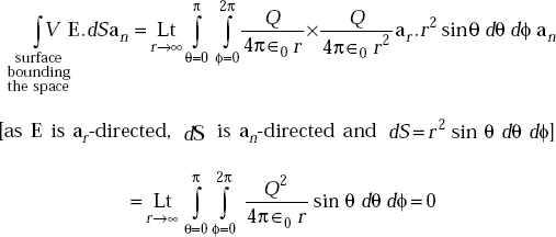
Hence Wt becomes
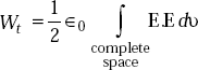
or,
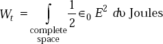
This expression is the total energy stored in an electrostatic field. Therefore, the integrand represents energy density, that is,
The energy density,
2.52 ENERGY IN A CAPACITOR
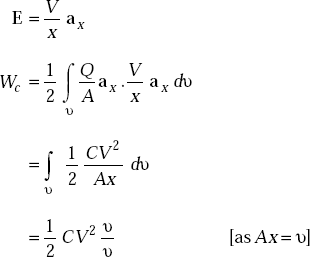
Energy stored in a capacitor is given by
Proof Method 1 We know that energy stored in the electric field of a capacitor is given by
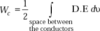
If the space between the conductors is occupied by a dielectric material whose relative permittivity is ∈r, then
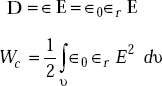
As the plates are assumed to be separated in x-direction,
and
Method 2 When a capacitor is charged, energy is stored in the electrostatic field which is set up in the dielectric medium.
Assume that a capacitor C is charged to a voltage, V. If the potential difference across the plates at any instant of charging is V, this is equal to the work done in shifting one coulomb of charge from one plate to another. If dQ is the charge transferred, work done is
As per the definition of C,
|
Q = CV |
|
dQ = C dV |
or, |
dWc = CV dV |
Total work done in producing a potential of V is
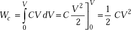
Energy stored in a capacitor
POINTS/FORMULAE TO REMEMBER
- Line charge density is Pl
- Surface charge density is
- Volume charge density,
- Coulomb’s law is
 , Newton.
 - ∈0 = 8.854× 10⁻¹², F/m
- F12 = –F21
- Displacement electric flux = electric flux = Q.
- Electric field intensity = electric field,

- E = –∇V,V/m
- Direction of Coulomb’s force is the same as electric field due to a point charge.
- Electric field due to a line charge is
- Electric field due to an infinite line charge is
- Electric field due to surface charge density,
- Electric field due to volume charge density,
- Potential at a point is
- Potential gradient, ∇V= –E.
- Potential due to electric dipole is
- Electric field due to a dipole is
- Electric flux, ψ = Q.
- Gauss’s law is
- Electric flux density,
- Point form of Gauss’s law is ∇.D = ρν.
- Laplace’s equation is ∇2 V = 0.
- Either Poisson’s or Laplace’s equation has unique solution.
- Etan1 = Etan2
- Dn1 — Dn2 = ρs
- Conduction current density, J c = σE.
- Displacement current density,

- Equation of continuity is

- Relaxation time,

- J = ρν V
- Electric dipole moment is p = Qd.
- Polarisation,
- Electric susceptibility,

- Displacement flux density in dielectrics is D = ∈ 0 E + P.
- Capacitance,
 Farad.
 - Capacitance of parallel capacitor,

- Capacitance of spherical condenser is
- Capacitance of a coaxial cable is
- Capacitance of parallel wires,
- Energy stored in electrostatic field is
- Energy stored in a capacitor,
 Joules.
OBJECTIVE QUESTIONS
1. Coulomb’s force depends on the medium in which the charges are placed. |
(Yes/No) |
2. Constant of proportionality in Coulomb’s law has units. |
(Yes/No) |
3. The directions of electric field and Coulomb’s force are the same. |
(Yes/No) |
4. For a thin filament extending from –∞ to ∞ along the z-axis, field varies with z and ϕ coordinates. |
(Yes/No) |
5. For a line charge extending from –∞ to ∞ along the z-axis, field at a point varies with ρ only. |
(Yes/No) |
6. For N point charges, the electric field at a point is the vectorial sum of the fields due to each of N charges. |
(Yes/No) |
7. Coulomb’s law can be applied to find electric field at a point. |
(Yes/No) |
8. Charge distributions produce electric field. |
(Yes/No) |
9. Electric field at a point due to a point charge is inversely proportional to r |
(Yes/No) |
10. Electric field at a point due to a point charge is proportional to 1/r2. |
(Yes/No) |
11. A surface of a conductor is an equipotential surface. |
(Yes/No) |
12. Gradient of the potential and equipotential surface are orthogonal to each other. |
(Yes/No) |
13. Electric dipole is a pair of two positive point charges. |
(Yes/No) |
14. Electric dipole is a pair of a positive charge and a negative charge. |
(Yes/No) |
15. Displacement electric flux is equal to the charge enclosed. |
(Yes/No) |
16. Faraday’s experiment says ψ = Q. |
(Yes/No) |
17. Gauss’s law is applicable on all surfaces. |
(Yes/No) |
18. Gauss’s law is applicable only on Gaussian surfaces. |
(Yes/No) |
19. Gauss’s law is applicable even if the charge is outside the closed surface. |
(Yes/No) |
20. Displacement flux depends on the dielectric material. |
(Yes/No) |
(Yes/No) |
|
22. Etan1 = Etan2 |
(Yes/No) |
23. Dn1 = Dn2 |
(Yes/No) |
24. Aluminium is a better conductor than silver at very low temperatures. |
(Yes/No) |
25. For a good conductor, |
|
26. Convection and conduction current densities are identical. |
(Yes/No) |
27. Convection current obeys Ohm’s law. |
(Yes/No) |
28. Conduction current obeys Ohm’s law. |
(Yes/No) |
29. Displacement current in a conductor is greater than conduction current, |
(Yes/No) |
30. Displacement current in dielectrics is greater than conduction current. |
(Yes/No) |
31. The current density, J = ρν V. |
(Yes/No) |
32. |
(Yes/No) |
33. |
(Yes/No) |
34. Electric dipole moment is a vector. |
(Yes/No) |
35. The polarisation, P = χe∈0 E. |
(Yes/No) |
36. Electric susceptibility has the unit of permittivity. |
(Yes/No) |
37. Electric susceptibility has no units. |
(Yes/No) |
38. Polarisation is a result of free electrons in dielectrics. |
(Yes/No) |
39. Polarisation is a result of bound electrons in dielectrics. |
(Yes/No) |
40. Electric flux density in dielectrics is greater than that in free space for field. |
(Yes/No) |
41. Capacitance depends on dielectric material between the conductors. |
(Yes/No) |
42. Gauss’s law can be applied on arbitrary Gaussian surfaces. |
(Yes/No) |
43. Potential is inversely proportional to r. |
(Yes/No) |
44. The unit of potential is Joule/Coulomb. |
(Yes/No) |
45. Potential obeys the superposition principle. |
(Yes/No) |
(Yes/No) |
|
47. Electrostatic energy is quadratic in the fields. |
(Yes/No) |
48. Electrostatic energy does not obey superposition principle. |
(Yes/No) |
49. |
|
50. E is perpendicular to the surface just outside a conductor. |
(Yes/No) |
51. ρν = 0 inside a conductor. |
(Yes/No) |
52. Charge resides on the surface of a conductor. |
(Yes/No) |
53. Direction of dipole moment is in the direction of applied electric field. |
(Yes/No) |
54. Coulomb’s force has the unit of _____. |
|
55. The unit of constant of proportionality in Coulomb’s law is _____. |
|
56. The unit of line charge density is _____. |
|
57. The unit of surface charge density is _____. |
|
58. The unit of volume charge density is _____. |
|
59. Electric field is defined as _____. |
|
60. The unit of electric field is _____. |
|
61. The unit of electric flux is _____. |
|
62. Laplace’s equation is _____. |
|
63. Relaxation time in dielectrics is _____. |
|
64. The unit of electric dipole moment is _____. |
|
65. The unit of polarisation of dielectric is _____. |
|
66. If ∈r = 3, electric susceptibility is _____. |
|
67. Application of electric field to dielectric material produces _____. |
|
68. Energy density in electric field is _____. |
|
69. Energy stored in a capacitor is _____. |
|
70. If the charge is doubled everywhere, the total energy is _____. |
|
71. Atomic polarisability has unit of _____. |
|
Answers
1. Yes |
2. Yes |
3. Yes |
4. No |
5. Yes |
6. Yes |
7. Yes |
8. Yes |
9. No |
10. Yes |
11. Yes |
12. Yes |
13. No |
14. Yes |
15. Yes |
16. Yes |
17. No |
18. Yes |
19. No |
20. No |
21. No |
22. Yes |
23. No |
24. Yes |
25. No |
26. No |
27. No |
28. Yes |
29. No |
30. Yes |
31. Yes |
32. No |
33. Yes |
34. Yes |
35. Yes |
36. No |
37. Yes |
38. No |
39. Yes |
40. Yes |
41. Yes |
42. Yes |
43. Yes |
44. Yes |
45. Yes |
46. Yes |
47. Yes |
48. Yes |
49. Yes |
50. Yes |
51. Yes |
52. Yes |
53. Yes |
54. Newton |
55. metre/Farad |
56. Coulombs/m |
57. C/m2 |
58. C/m3 |
59. E = –∇V |
60. V/m |
61. Coulomb |
62. ∇2 V = 0 |
63. ∈ /σ |
64. C–m |
65. C/m2 |
66. χe = 2 |
67. Induced dipole moment |
68. 0.5∈ E2 |
69. 0.5 CV2 |
70. Quadrupled |
71. Farad–m2 |
|
MULTIPLE CHOICE QUESTIONS
- Coulomb’s force is proportional to
- r
- r2


- The proportionality constant in Coulomb’s law has unit of
- Farads
- Farads/metre
- Newton
- metre/Farad
- The value of proportionality constant in Coulomb’s law is
- 9 × 10⁹
- 9 × 10⁻⁹
- 8.854 × 10⁻¹²

- The unit of electric field is
- Newton
- Coulomb/Newton
- Newton/Coulomb
- Coulomb/metre
- If the direction of Coulomb’s force on a unit charge is ax, the direction of electric field is
- –ax
- ay
- ax
- az
- The unit of electric flux is
- Coulomb
- Coulomb/metre
- Weber
- Weber/m2
- The electric field on x-axis due to a line charge extending from –∞ to ∞ is
- Electrostatic field due to a dipole consists of


- r terms
- Potential at all the points on the surface of a conductor is
- the same
- not the same
- zero
- infinity
- Gradient of the potential and an equipotential surface
- have the same direction
- have opposite directions
- are orthogonal to each other
- have no directional relation
- The potential at a point due to electric dipole consists of
- r terms


- The unit of electric dipole moment is
- C/m
- C-m
- C/m2
- C-m2
- The unit of polarisation in dielectric is
- C/m2
- C/m
- C/m3
- C-m2
- Point form of Gauss’s law is
- ∇.D = ρv
- ∇.D = ρs
- ∇.D = ρv/∈0
- ∇.D = Q
- The Laplacian operator, ∇2
- has unit of m2
- is a vector operator
- has unit of 1/m2
- has no unit
- Laplace’s equation has
- two solutions
- infinite solutions
- no solution
- only one solution
- The surface charge density in a good dielectric is
- zero
- ρs
- infinity
- – ρs
- Relaxation time of a medium with ∈r = 3.0 and σ = 3.0 Mho/m is
- 8.854 picosecond
- 9 picosecond
- 7.9686 picosecond
- 1 second
- The force magnitude between Q1 = 1C and Q2 = 1C when they are separated by 1 m in free space is
- 9 × 10⁹ N
- 8.854 × 10⁻¹² N
- 9 × 1–9 N
- When the force on 2 C due to fixed charge of 4 C is 2 N, the electric field at the charge of 2 C is
- If ∈r = 2 for a dielectric medium, its electric susceptibility is
- 1
- 2
- 3
- 2∈0
- If a pair of (+)ve and (-)ve charges of 1 C each are separated by a distance of 1.0 μm, the magnitude of dipole moment is
- 2 C-μm
- 1 C-μm
- 0 C-μm
- 1 C-μm
- If dipole moment of 1 C-m in a dielectric material of volume 0.1 m3 exists, the polarisation is
- 10 C/m2
- 0.1 C/m2
- 10 C/m
- 0.1 C/m
- If a charge element, whose volume charge density is 2.0 C/m2, is moving with a velocity of 3ax m/s, the current density is
- 6ax A/m2
- 6ax A/m
- 1.5ax A/m2
- 1.5ax A/m
- If Etan1 = ax and En1 = 0, the electric field E2 in a dielectric medium 2 is
- ax
- 2ax
- ay
- az
- Two point charges Q1 = 1 C and Q2 = 3 C are separated by 1.0 m. The force on Q1 is
- zero
- repulsive
- attractive
- increasing linearly
- A charge density of 10 nC/m2 is distributed on a plane z = 10 m, the electric field intensity at the origin is
- – 180π az V/m
- – 10π az V/m
- – 360π az V/m
- – 18π az V/m
- If a force, F = 4ax + ay + 2az moves 1μC charge through a displacement of 4ax + 2ay – 6az, the resultant work done is
- 6 μ J
- 12 μ J
- 18 μ J
- 24 μ J
- If a potential of 1 V is applied across a capacitor of 10 PF, the energy stored is
- 5 PJ
- 10 PJ
- 100 PJ
- 0.01 PJ
- Example of non-polar type of dielectric is
- water
- hydrochloric acid
- sulphur dioxide
- oxygen
- Example of polar type of dielectric is
- oxygen
- water
- hydrogen
- nitrogen
- If the voltage applied across a capacitor is increased, the capacitance value
- increases
- decreases
- remains constant
- becomes infinity
- If the electric field intensity is 1 V/m in free space, the energy density is
- 4.427 PJ/m3
- 8.854 PJ/m3
- 4.427 PJ
- 8.854 PJ
- If electric susceptibility of a dielectric is 4, its relative permittivity is
- 5
- 4
- 3
- 2
- The unit of electric flux is
- Coulomb
- Coulomb/m
- Weber
- Tesla
- Gauss’s law is
- Gauss’s law in point form is
- ∇.D = ρv
- ∇.D = ρs
- ∇.D = Q
- ∇D = ρv
- Equation of continuity is
- Relaxation time is
- In dielectrics,
- Potential has the unit of
- Joules/Coulomb
- Joules
- Joules/m3
- Joules/m2
- If a total charge of 10 coulombs is uniformly distributed along a filament of length 10 m, the line charge density is
- 1 C/m
- 100 C-m
- 100 C/m
- 1 C-m
- If a charge of 10 coulombs is uniformly distributed on the surface of a conductor of area 10 m2, the surface charge density is
- 1 C/m2
- 100 C/m2
- 1 C-m2
- 100 C-m2
- If a total charge of 1 C is contained in a tiny sphere of volume 0.1 m3, the volume charge density is
- 10 C/m3
- 0.1 C/m3
- 10 C-m3 Q
- 10 C/m2 Q
- Electric flux density is
- Poisson’s equation is
- ∇2 V = ρv / ∈
- ∇2 V = −ρv / ∈
- ∇2 V = −ρv
- Boundary condition for the normal component of E on the boundary of a dielectric is
- En1 = En2
- En1 – En2 = ρs
- En1 = 0
- Electric flux lines
- Unit of electric flux is
- Coulomb
- Weber
- Tesla
- Weber/m
- Potential due to a charge at a point situated at ∞ is
- zero
- ∞
- –∞
- 1
Answers
1. (d) |
2. (d) |
3. (a) |
4. (c) |
5. (c) |
6. (a) |
7. (a) |
8. (c) |
9. (a) |
10. (c) |
11. (b) |
12. (b) |
13. (a) |
14. (a) |
15. (c) |
16. (d) |
17. (a) |
18. (a) |
19. (a) |
20. (a) |
21. (a) |
22. (d) |
23. (a) |
24. (a) |
25. (a) |
26. (b) |
27. (a) |
28. (a) |
29. (a) |
30. (d) |
31. (b) |
32. (c) |
33. (a) |
34. (a) |
35. (a) |
36. (b) |
37. (a) |
38. (b) |
39. (a) |
40. (d) |
41. (a) |
42. (a) |
43. (a) |
44. (a) |
45. (a) |
46. (b) |
47. (c) |
48. (a) |
49. (a) |
50. (a) |
||
EXERCISE PROBLEMS
- An infinite line charge, ρL = 10 nC/m parallel to z-axis is at x = 3, y = 4 in free space. Find E at
- (0, 0, 0)
- (0, 1, 2)
- (1, 1, 1)
- Determine the force on a point charge of 5 nC at (0, 0, 5) m due to uniformly distributed charge of 5 mC over a circular disc of radius r ≤ 1 m in z = 0 plane.
- Find the total charge in the volume specified by 0 ≤ x ≤ 1 m, 0 ≤ y ≤ 1 m and 0 ≤ z ≤ 1 m when ρv = 30x2 y (nC/m3).
- Three infinitely long lines charged uniformly are parallel to the z-axis. They are separated by a distance of b m. The charge density of each is ρL = 2.0 PC/m. Find the electric field E at a point P on the y-axis at y = a m. If a = b = 1 m, what is the electric field, E?
- A dipole consists of two charges Q and – Q separated by 2b m as shown in Fig. 2.34. Determine the electric field at point P.
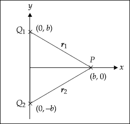
Fig. 2.34
- An infinite length of uniform line charge has ρL = 10 PC/m and it lies along the z-axis. Determine electric field E at (4, 3, 3) m.
- When six equal charges Q = 10 PC are located at (2, 0, 0), (3, 0, 0), (4, 0, 0), (5, 0, 0), (6, 0, 0) and (7, 0, 0), find the potential at the origin.
- If the electric potential is as shown in Fig. 2.35, sketch the respective electric field distribution in a specified region.
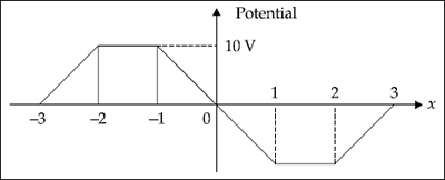
Fig. 2.35
-
- What is the force magnitude between two charges Q1 = 4 nC and Q2 = 6 nC which are separated by 0.1 m in free space.
- What will happen if they are kept in ice whose ∈r = 4.2?
- Consider the Fig. 2.36.
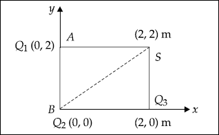
Fig. 2.36
If Q1 = 4 nC, Q2 = 4 nC, Q3 = 4 nC, find the electric field at point S. Assume that the charges are in free space.
- Two point charges Q1 = 5.0 nC and Q2 = 1.0 nC are located at (– 1, 1, –3) m and (3, 1, 0) m respectively. Determine the electric field at Q1 and Q2.
- An electric field is given by E = 10yax + 10xay, V/m. Find the potential function, V. Assume V = 0 at the origin.
- Consider concentric spherical shells in free space in which V = 0 at r = 10 cm and V = 10 volts at r = 20 cm. Find E and D.
- If electric flux density, D is given by D = [(2y2 + z)ax + 4xyay + xaz)] mC/m2, find the volume charge density at (0, 0, 0) and (–1, 0, 4).
- A sphere whose radius is 0.5 m contains a charge density of ρv = (5 – 2r)mC/m3. Find D at a distance 10 m away from the centre of the sphere.