Chapter 2
Fourier’s Law and Its Consequences
2.1 Introduction
While studying the subject of heat transfer, one of our objectives is to calculate the rate of heat transfer. From the second law of thermodynamics, we know that there must be a temperature gradient for heat transfer to occur, i.e. heat flows from a location of high temperature to a location of low temperature. Fourier’s law gives the relation between the rate of heat flow and temperature gradient and is therefore considered to be the fundamental law of conduction.
In this chapter, we will first study Fourier’s law and the assumptions behind this law. Then, follow two important consequences of Fourier’s law; the first one being the definition of thermal conductivity—an important transport property of matter, and the second one being the concept of thermal resistance. We will study about the thermal conductivity of solids, liquids and gases and the variation of this property with temperature. Thermal resistance concept simplifies the solution of many practical problems of steady state heat transfer with no internal heat generation, but involving heat transfer through multiple layers or when different modes of heat transfer occur simultaneously.
2.2 Fourier’s Law of Heat Conduction
This is the basic rate equation for heat conduction which gives a relation between the rate of heat transfer and the temperature gradient.
Fourier’s law states that one-dimensional, steady state heat flow rate between two isothermal surfaces is proportional to the temperature gradient causing the heat flow and the area normal to the direction of heat flow.
Referring to Fig. 2.1, we get,
where, |
Q = heat flow rate in X-direction, W |
|
A = area normal to the direction of heat flow (note this carefully), m2 |
dT/dx = temperature gradient, deg./m
k = thermal conductivity, a property of the material, W/(mC) or W/(mK)
This is the differential form of Fourier’s equation written for heat transfer in the X-direction. Negative sign in Eq. 2.2 requires some explanation. We know that heat flows from a location of higher temperature to a location of lower temperature. Referring to Fig. 2.1, if the heat flow rate Q has to occur in the positive X-direction, temperature has to decrease in the positive X-direction, i.e. temperature must decrease as X increases; this means that temperature gradient dT/dx is negative. Since we would like to have the heat flowing in the positive X-direction to be considered as positive, a negative sign is inserted in Eq. 2.2, so that Q becomes positive.
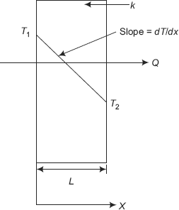
FIGURE 2.1 Fourier’s law
Let us state succinctly the assumptions and other salient points regarding the Fourier’s law:
- Fourier’s law is an empirical law, derived from experimental observations and not from fundamental, theoretical considerations.
- Fourier’s law is defined for steady state, one-dimensional heat flow.
- It is assumed that the bounding surfaces between which heat flows are isothermal and that the temperature gradient is constant, i.e. the temperature profile is linear.
- There is no internal heat generation in the material.
- The material is homogeneous (i.e. constant density) and isotropic (i.e. thermal conductivity is the same in all directions).
- Fourier’s law is applicable to all states of matter, i.e. solid, liquid or gas.
- Fourier’s law helps to define thermal conductivity i.e. from Eq. 2.2 we can write, for steady state heat transfer through a slab of thickness L and its two surfaces at constant temperatures of T1 and T2, (T1 > T2).
Q = −kA dT/dx= −kA (T2 − T1)/L= kA (T1 − T2)/L
We can say that
Q = <k> when A = 1 m2, dT = 1 deg., dx = 1 m,
i.e. thermal conductivity of a material is numerically equal to the heat flow rate through an area of one m2 of a slab of thickness 1 m with its two faces maintained at a temperature difference of one degree celcius.
Therefore, the unit of thermal conductivity is obtained from:
Note that W/(mC) and W/(mK) mean the same thing in Eq. 2.3, (T1 – T2) is the temperature difference which is the same whether it is deg.C or deg.K.
2.3 Thermal Conductivity of Materials
We state Fourier’s law again:
Here, k is the thermal conductivity, a property of the material. Its units: W/(mC) or W/(mK). Thermal conductivity, essentially depends upon the material structure (i.e. crystalline or amorphous), density of material, moisture content, pressure and temperature of operation.
Thermal conductivity of materials varies over a wide range, by about 4 to 5 orders of magnitude. For example, thermal conductivity of Freon gas is 0.0083 W/(mC) and that of pure silver is about 429 W/(mC) at normal pressure and temperature.
Fig 2.2 shows the range of variation of thermal conductivity of different classes of materials:
Table 2.1 gives values of thermal conductivities for a few materials at room temperature.
2.3.1 Thermal Conductivity of Solids
Thermal conductivity of solids is made up of two components,
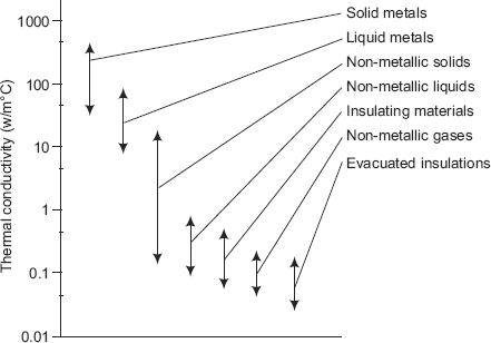
FIGURE 2.2 Range of thermal conductivities of various materials
- due to flow of free electrons, and
- due to lattice vibrations.
First effect is known as electronic conduction and the second effect is known as phonon conduction.
2.3.1.1 Metals and Alloys.
In case of pure metals and alloys,
- There is an abundance of free electrons and the electronic conduction predominates. Since free electrons are also responsible for electrical conduction, it is observed that good electrical conductors are also good thermal conductors, e.g. copper, silver etc.
- Any effect which inhibits the flow of free electrons in pure metals reduces the value of thermal conductivity. For example, with a rise in temperature, the lattice vibration increases and this offers a resistance to the flow of electrons and therefore, for pure metals thermal conductivity decreases as temperature increases (uranium and aluminium are exceptions). Fig. 2.3 shows the variation of thermal conductivity with temperature for a few metals.
TABLE 2.1 Thermal conductivity of a few materials at room temperature
Material k, W/mC Diamond
2300
Silver
429
Copper
401
Gold
317
Aluminium
237
Iron
80.2
Mercury (l)
8.54
Glass
0.78
Brick
0.72
Water (l)
0.613
Wood (oak)
0.17
Helium (g)
0.152
Refrigerant-12
0.072
Glass fibre
0.043
Air (g)
0.026
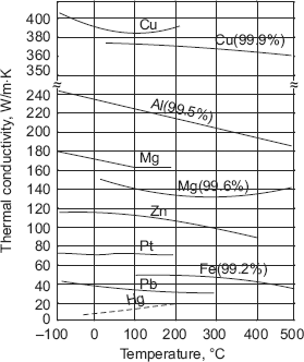
FIGURE 2.3 Variation of thermal conductivity with temperature for a few metals
- Alloying decreases the value of thermal conductivity since the foreign atoms cause scattering of free electrons, thus impeding their free flow through the material. For example, thermal conductivity of pure copper near about room temperature is 401 W/(mC) while presence of traces of arsenic reduces the value of thermal conductivity to 142 W/ (mC).
- Heat treatment, mechanical forming and cold working reduce the value of thermal conductivity of pure metals.
- Thermal conductivity of alloys generally increases as temperature increases. Fig. 2.4 below confirms this trend for a few alloys.
- Since the phenomenon of electron conduction is responsible for both thermal conduction and electrical conduction, it is reasonable to presume that there must be relation between these two quantities. In fact, Weidemann–Franz law gives this relation. This law, based on experimental results, states the ratio of thermal and electrical conductivities is the same for all metals at the same temperature and this ratio is directly proportional to the absolute temperature of the metal.

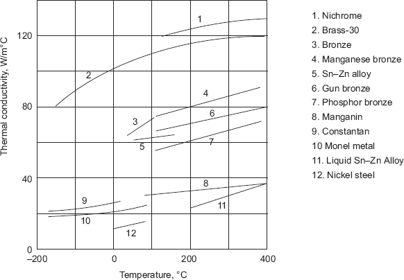
FIGURE 2.4 Variation of thermal conductivity with temperature for a few alloys
where |
k = thermal conductivity of metal, W/(mK) |
|
σ = electrical conductivity of metal, (ohm.m)–1 |
|
C = Lorentz number, a constant for all metals |
|
= 2.45 × 10⁻⁸ W Ohms/K2 |
An important practical application of Weidemann–Franz law is to determine the value of thermal conductivity of a metal at a desired temperature, knowing the value of electrical conductivity at the same temperature. Note that it is easier to measure experimentally the value of electrical conductivity than that of thermal conductivity.
2.3.1.2 Non-metallic Solids.
In case of non-metallic solids,
- For dielectrics, there are no free electrons and the thermal conductivity values are much lower than those of metals. For heat insulating materials, general range of values of k are from 0.023 W/(mC) to 2.9 W/(mC). Thermal conductivity increases with temperature for insulating materials as shown in Fig. 2.5.
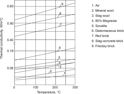
FIGURE 2.5 Variation of thermal conductivity with temperature for insulating materials
- For porous heat insulating materials (brick, concrete, asbestos, slag, etc.), thermal conductivity depends greatly on density of the material and the type of gas filling the voids. For example, k of asbestos increases from 0.105 to 0.248 W/(mC) as density increases from 400 to 800 kg/m3; is due to the fact that thermal conductivity of air filling the voids is much less than that of the solid material.
- Thermal conductivity of porous materials also depends on the moisture content in the material; k of a damp material is much higher than that of the dry material and water taken individually.
- Thermal conductivity of granular materials increases with temperature since with increasing temperature, radiation from the granules also comes into picture along with conduction of medium filling the spaces.
- Variation of thermal conductivity of solids with temperature: In heat transfer calculations, generally we assume k to be constant when the temperature range is small; however, when the temperature range is large, it is necessary to take into account the variation of k with temperature.
Usually, for solids, a linear variation of thermal conductivity with temperature can be assumed without loss of much accuracy.
where, |
k(T) = thermal conductivity at desired temperature T, W/(mC) |
|
k0 = thermal conductivity at reference temperature of 0°C, W/(mC) |
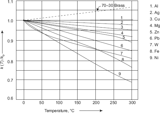
FIGURE 2.6 Variation of thermal conductivity with temperature for a few pure metals
TABLE 2.2 Representative values of k0 and β in Eq. 2.5
| Material | k0 (W/mC) | β × 104, (1/C) |
|---|---|---|
Metals and alloys |
|
|
Aluminium |
246.985 |
– 2.227 |
Chromium |
97.123 |
– 5.045 |
Copper |
401.5275 |
– 1.681 |
Stainless steel |
14.695 |
+ 10.208 |
Uranium |
26.679 |
+ 8.621 |
Insulators |
|
|
Fireclay brick |
0.76 |
0.895 |
Red brick |
0.56 |
0.66 |
Sovelite |
0.092 |
0.12 |
85% Magnesia |
0.08 |
0.101 |
Slag wool |
0.07 |
0.101 |
Mineral wool |
0.042 |
0.07 |
β = a temperature coefficient, 1/C
T = temperature, °C
Fig. 2.6 shows the variation of k with temperature for a few pure metals. It may be noted that the variation is linear as indicated in Eq. 2.5.
In Eq. 2.5, value of β may be positive or negative. Generally, β is negative for metals (exception being uranium) and positive for insulators and alloys. Table 2.2 gives representative values of k0 and β for a few materials.
2.3.2 Thermal Conductivity of Liquids
2.3.2.1 Non-metallic Liquids.
Heat propagation in liquids is considered to be due to elastic oscillations. As per this hypothesis, the thermal conductivity of liquids is given by,
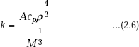
where, |
cp = specific heat of liquid at constant pressure |
|
ρ = density of liquid |
|
M = molecular weight of liquid |
|
A = constant depending on the velocity of elastic wave propagation in the liquid; it does not depend on nature of liquid, but on temperature. |
It is noted that the product A.cp is nearly constant. As temperature rises, density of a liquid falls and as per Eq. 2.6 the value of thermal conductivity also drops for liquids with constant molecular weights. (i.e. for non-associated or slightly associated liquids). This is generally true as shown in Fig. 2.7.
Notable exceptions are water and glycerin, which are heavily associated liquids. With rising pressure, thermal conductivity of liquids increases. For liquids, k value ranges from 0.07 to 0.7 W/(mC).
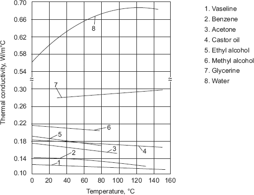
FIGURE 2.7 Thermal conductivity of non-metallic liquids
2.3.2.2 Liquid Metals.
Liquid metals like sodium, potassium etc. are used in high flux applications as in nuclear power plants where a large amount of heat has to be removed in a small area. Thermal conductivity values of liquid metals are much higher than those for non-metallic liquids. For example, liquid sodium at 644 K has k = 72.3 W/ (mK); liquid potassium at 700 K has k = 39.5 W/(mK); and liquid bismuth at 589 K has k = 16.4 W/(mK).
2.3.3 Thermal Conductivity of Gases
- Heat transfer by conduction in gases at ordinary pressure and temperature is explained by the Kinetic Theory of Gases. Temperature is a measure of kinetic energy of molecules. Random movement and collision of gas molecules contribute to the transport of kinetic energy, and, therefore, to transport of heat. So, the two quantities that come into picture now are: the mean molecular velocity, V and the mean free path, l. Mean free path is defined as the mean distance travelled by a molecule before it collides with another molecule.
Thermal conductivity of gases is given by,
where,
V = mean molecular velocity
l = mean free path
cv = specific heat of gas at constant volume
ρ = density
- As pressure increases, density ρ increases, but the mean free path l decreases almost by the same proportion and the product l ρ remains almost constant, i.e the thermal conductivity of gases does not vary much with pressure except at very low (less than 20 mmHg) or very high (more than 20,000 bar) pressures.
- As to the effect of temperature on thermal conductivity of gases, mean molecular velocity V depends on temperature as follows,

where
G = Universal gas constant = 8314.2 J/kmol K
M = molecular weight of gas
T = absolute temperature of gas, K
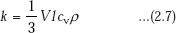
i.e. mean molecular velocity varies directly as the square root of absolute temperature and inversely as the square root of molecular weight of a gas. Specific heat, cv also increases as temperature increases. As a result, thermal conductivity of gases increases as temperature increases.
- For the reason stated above, gases with lower molecular weights such as helium and hydrogen have higher values of thermal conductivities (almost by 5 to 10 times) as compared to gases with higher molecular weights such as air.
- Generally, thermal conductivity values for gases vary in the range 0.006 to 0.6 W/(mC)
- Thermal conductivity of steam and other imperfect gases depend very much on pressure unlike that of perfect gases.
Fig. 2.8 and Fig. 2.9 show the variation of k with temperature for a few gases.
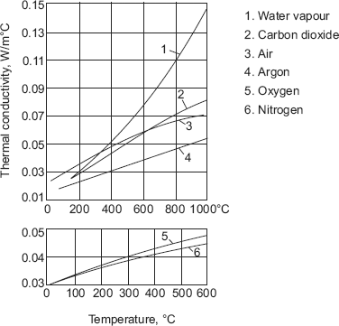
FIGURE 2.8 Variation of k with temperature for a few gases
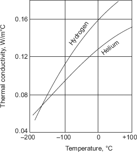
FIGURE 2.9 Variation of k with temperature for hydrogen and helium
2.3.4 Insulation Systems
It is appropriate here to consider insulation systems generally used. In industries where huge amount of thermal energy is dealt with, be it for high temperature or low temperature application, it is necessary to see that the most suitable insulation is adopted. This has become particularly important now, since there is widespread awareness about the energy crunch and the cost of energy.
Insulation is required for high temperature systems as well as low temperature systems. In high temperature systems, any leakage of heat from boilers, furnaces or piping carrying hot fluids represents an energy loss. Similarly, in low temperature/cryogenic systems, any heat leakage into the low temperature region represents an energy loss since from thermodynamics we know that to pump out a given amount of heat from a low temperature region would need a disproportionately large amount of work to be put in at room temperature.
Insulation systems may be classified as,
- fibrous
- cellular
- powder
- reflective.
Since in non-homogeneous insulation materials, a combination of conduction, convection or radiation is involved, they are characterised by an “effective thermal conductivity”. Solid materials have cells of spaces formed inside them by foaming. There may be air or some other gas inside these voids. Type of gas used affects the property of the material. Obviously, density of these systems plays an important role in determining the effective thermal conductivity. Sometimes, the intervening spaces are evacuated to reduce the convection losses. To get extremely low values of thermal conductivity—of the order of a few μW/(mK)—multiple layers of highly reflective materials are introduced in between the insulation layers. These are called superinsulations and are used in cryogenic and space applications.
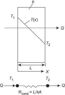
FIGURE 2.10 Conduction heat flow through a slab—thermal resistance
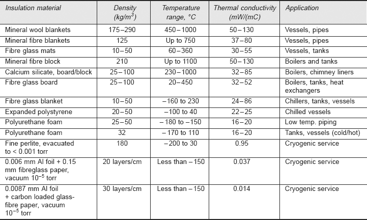
Table 2.3 gives details about some of the common insulations used in industry.
TABLE 2.3 Common Insulations used in Industry
2.4 Concept of Thermal Resistance
2.4.1 Conduction
Consider a slab of thickness L, constant thermal conductivity k, with its left and right faces maintained at temperatures T1 and T2. If T1 is greater than T2, we know that heat will flow from left to right and the heat flow rate is given by Fourier’s law,
Now, consider this: in a pipe carrying a fluid, the flow occurs under a driving potential of a pressure difference and there is resistance to flow due to pipe friction; in an electrical conductor, flow of electricity occurs under the driving potential of a voltage difference and there is a resistance to the flow of electric current. Similarly, considering Eq. 2.9, we can say that flow of heat Q occurs in the slab by conduction under a driving potential of a temperature difference (T1 – T2) and the material offers a thermal resistance to the flow of heat. So, we can write Eq. 2.9 as,
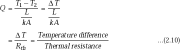
Rth L/(kA) is known as Thermal resistance of the slab for conduction.
It is seen that there is a clear analogy between the flow of heat and flow of electricity, as shown below,

Fig. 2.10 above shows the thermal circuit for the situation of flow of heat through a plane slab by conduction. For the slab, we write,
Note that units of thermal resistance is (C/W) or, K/W.
2.4.2 Convection
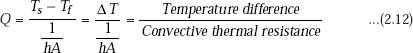
Consider the case of a fluid flowing with a free stream velocity U and free stream temperature Tf, over a heated surface maintained at a temperature Ts. Let the heat transfer coefficient for convection between the surface and the fluid be h. Then, the heat transfer rate from the surface to the fluid is given by Newton’s rate equation,
This can be written as,
Again, note the analogy between flow of electricity and the flow of heat (see Fig. 2.11).
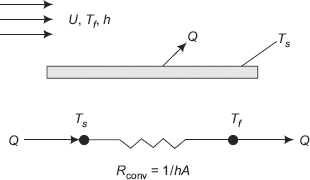
FIGURE 2.11 Convection heat transfer — thermal resistance
So, for heat transfer by convection, we write,
Note that the units are (C/W) or (K/W).
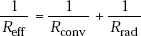
2.4.3 Radiation
For the case of heat transfer between two finite surfaces, at temperatures T1 and T2 (Kelvin), net radiation heat transfer between them is given by equation,
where, F1 is known as shape factor or view factor, which includes the effects of orientation, emissivities and the distance between the surfaces. s is the Stefan–Boltzmann constant.
Write the above equation in the following form,

Clearly, the radiation thermal resistance may be written as,
2.4.4 Practical Applications of Thermal Resistance Concept
There are two important practical application of the thermal resistance concept:
- To analyse the problems where one or more modes of heat transfer occur simultaneously. For example, in a heat exchanger plate when a hot fluid flows on one side and a cold fluid on the other side, we have heat transfer occurring at either surface by convection and through the plate itself by conduction. Obviously, the thermal resistances in this case are all in series and the rules of series resistances in an electrical circuit apply, i.e. total thermal resistance is the sum of the three resistances.
i.e. Reff = Rconv1 + Rcond + Rconv2
But in some other cases, the thermal resistances may be in parallel; for example, a heated wall of a furnace may lose heat to ambient by convection as well as radiation, i.e. heat transfer occurs from the wall by these two modes simultaneously in parallel. Then we apply the rule for parallel resistances, i.e. effective resistance is given by,
- To analyse the problems where multiple layers of materials of different thermal conductivities are used; e.g. in furnace walls which are lagged with 2 or 3 layers of insulation, insulation of walls of houses in cold weather, lagging of pipes, etc. Since the thermal conductivities and thicknesses of materials used may be different, thermal resistances of individual layers are different and it becomes convenient to use the thermal resistance concept to find out the total resistance and hence the heat flow rate.
2.4.5 Limitations for the Use of Thermal Resistance Concept
Thermal resistance concept can be used only when all the following conditions are satisfied.
- One-dimensional conduction
- Steady state conduction
- No internal heat generation.
Note: In this chapter, we have just introduced the concept of thermal resistance. We will study more about this concept and apply it to analyse heat transfer in composite slabs, cylinders and spheres and also to situations where more than one mode of heat transfer exist simultaneously, in Chapter 4. Therein, we shall also solve several numerical problems to illustrate the applications of this concept.
2.5 Thermal Diffusivity (α)
Often, during heat transfer analysis, particularly while dealing with transient conduction problems, we come across a quantity called Thermal diffusivity, defined as,
where, |
k = thermal conductivity of the material, W/(mC) |
|
ρ = density, kg/m3 |
|
cp = specific heat at constant pressure, J/(kg.C) |
Note that unit of α is m2/s.
Let us consider the physical significance of thermal diffusivity, α: Thermal conductivity (k) of a material is a transport property and denotes its ability to conduct heat; higher the value of k, better the ability of material to conduct heat. The product (ρ cp) is known as volumetric heat capacity, has units of J/(m3K), and denotes the ability of the material to store heat. Higher the value of (ρcp), larger the heat storage capacity. Generally, solids and liquids which are good storage media have higher volumetric heat capacity (> 1 MJ/m3 K) as compared to gases (about 1 kJ/m3 K), which are poor heat storage media. Therefore, thermal diffusivity, i.e. the ratio of k to (ρcp) gives the relative ability of the material to conduct heat as compared to its ability to store heat. Larger the value of α, faster the propagation of heat into the material. In other words, α represents the ability of the material to respond to changes in the thermal environment; larger the value of α, quicker the material will come into thermal equilibrium with its surroundings. Values of α for materials vary over a wide range. For example, for copper at room temperature, its value is approx. 113 × 10−6 m2/s, whereas for glass it is about 0.34 × 10⁻⁶ m2/s.
Table 2.4 shows typical values of thermal diffusivity for a few materials.
2.6 Summary
In this chapter, we studied Fourier’s law for one-dimensional conduction. This is a very important topic and student must be clear about the assumptions behind this law; particularly, you should note that the area used in applying this law is the area normal to the direction of heat flow. Fourier’s law opens the door for further learning about conduction; we will use it immediately in the next chapter to derive the general differential equation for conduction heat transfer. In this chapter, we also studied two important consequences of Fourier’s law: firstly, definition of thermal conductivity—an important transport property of material—and, secondly, concept of thermal resistance. We studied in some detail about the thermal conductivity of solids, liquids and gases and the variation of thermal conductivity with temperature. Thermal diffusivity—a significant property while studying transient conduction—was mentioned and its physical significance explained.
TABLE 2.4 Typical values of thermal diffusivity (α) for a few materials at room temperature
| Material | α × 106, (m2/s) |
|---|---|
Silver |
149 |
Gold |
127 |
Copper |
113 |
Aluminium |
97.5 |
Iron |
22.8 |
Mercury (l) |
4.7 |
Marble |
1.2 |
Ice |
1.2 |
Concrete |
0.75 |
Brick |
0.52 |
Glass |
0.34 |
Glasswool |
0.23 |
Water (l) |
0.14 |
Beef |
0.14 |
Wood (oak) |
0.13 |
In the next chapter, we shall derive the general differential equation for conduction which, when solved, will give the temperature distribution in a material; knowing the temperature distribution, we can easily determine the heat transfer rate by applying the Fourier’s law.
Questions
- State and explain Fourier’s law for one-dimensional conduction. What are the underlying assumptions?
- What are the important consequences of Fourier’s law?
- Define ‘thermal conductivity’. What are the factors affecting the thermal conductivity of a material?
- Write a short note on thermal conductivity of solids, liquids and gases.
- How does thermal conductivity vary with temperature for metals, alloys and insulators?
- Name the different insulations used in industry and mention the specific purpose for which each is used.
- Explain the analogy between flow of heat and flow of electricity.
- Explain the concept of thermal resistance. What are the practical uses of this concept?
- What do you understand by the term ‘thermal diffusivity’? Explain its physical significance.
- On a cold, winter morning, the aluminium handle of the front door of your house feels cold to touch as compared to the wooden door frame, even though both were exposed to the same cold environment throughout the night. Explain why?
- The inner and outer surfaces of a 5 m × 6 m brick wall of thickness 30 cm and thermal conductivity 0.69 W/(mC), are maintained at temperatures of 20°C and 35°C, respectively. Determine the rate of heat transfer through the wall.
- In an experiment to find out the thermal conductivity of a material, an electric heater is sandwiched between two identical samples, each of size (10 cm × 10 cm) and thickness 0.5 cm, and all the four outer edges are well insulated. At steady state, it is observed that the electric heater draws 35 W of power and the temperature of each sample was 90°C on the inner surface and 82°C on the outer surface. Determine the thermal conductivity of the material at the average temperature.
- By conduction, 3 kW of energy is transferred through 0.5 m2 section of a 5 cm thick insulating material of thermal conductivity 0.2 W/(mC). Determine the temperature difference across the layer.