Chapter 4
One-dimensional Steady State Heat Conduction without Heat Generation
4.1 Introduction
In this chapter, we shall take up the study of one-dimensional, steady state heat conduction, without heat generation in a few common geometries such as plane slab, cylindrical shell and spherical shell. By one-dimensional conduction, we mean that temperature variation is significant only in one-dimension and is negligible in other dimensions; and, steady state means that the temperature does not vary with time at any location. Obviously, solution of differential equation governing one-dimensional conduction will be much easier than that of the general differential equation for three-dimensional conduction.
There are many practical instances where the heat conduction may be considered to be one-dimensional, e.g. a plane slab whose thickness is small as compared to its length and breadth may be considered to have its temperature varying only along its thickness; temperature in a long, cylindrical shell may be considered to be varying only along its radius etc.
Solution of the governing differential equation along with the boundary conditions gives the temperature field within the material and then, by applying Fourier’s law, we can calculate the heat flux at any point.
We shall, first, study heat transfer in three common, important geometries, namely plane slab, cylindrical and spherical systems, with thermal conductivity of the material remaining constant. Plane slab is an important case, applicable to analysis of heat transfer in boiler walls, furnace walls, and walls of buildings etc. Cylindrical geometry is extremely popular for piping, containers etc. along with their insulations. Similarly, sphere is a popular geometry used in industry to store hot/cold liquids, gases, chemicals etc.
We will also study heat transfer through multiple layers in these three geometries applying the thermal resistance concept, already mentioned in the second chapter. We shall derive expressions for overall heat transfer coefficient which is very useful in study of heat exchangers. We shall also present the concept of critical thickness of insulation and optimum thickness of insulation and study their practical applications.
We shall, next, examine the heat transfer and temperature distribution in these geometries when the thermal conductivity of the material varies with temperature.
Finally, we shall study briefly about two-dimensional conduction and present values of shape factors for a few common situations.
4.2 Plane Slab
Consider a plane slab as shown in Fig. 4.1. Let the thickness be L. Temperatures at the two faces are constant and uniform, i.e. T = T1 at x = 0 and T = T2 at x = L.
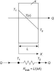
FIGURE 4.1 Plane slab and thermal circuit
Assumptions:
- One-dimensional conduction, i.e. thickness L is small compared to the dimensions in the y and z-directions.
- Steady state conduction, i.e. temperature at any point within the slab does not change with time; of course, temperatures at different points within the slab will be different.
- No internal heat generation.
- Material of the slab is homogeneous (i.e. constant density) and isotropic (i.e. value of k is same in all directions).
Our problem is to find out the temperature field within the slab and then the heat flux at any point.
We start with the general differential equation in Cartesian coordinates, since the geometry under consideration is a slab, we have from eqn. (3.9):
In this case, ![]() since one-dimensional conduction, i.e. temperature gradients are zero in y and z-directions
since one-dimensional conduction, i.e. temperature gradients are zero in y and z-directions
|
|
|
qg |
= |
0, since there is no internal heat generation |
kx |
= |
ky = kz = k, say, since the material is isotropic and not dependent on temperature. |
So, the governing equation for the plane slab with the above-mentioned assumptions becomes:
i.e.
Temperature field is obtained by solving Eq. 4.2.
Integrating Eq. 4.2 once:
Integrating again:
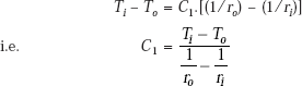
Eq. 4.3 is the general solution for the temperature distribution. Values of the two integration constants C1 and C2 are obtained from the two boundary conditions, namely,
B.C.(i): T = T1 at x = 0 |
|
B.C.(ii): T = T2 at x = L |
|
From B.C.(i) and Eq. 4.3: |
T(0) = T1 = C2 |
From B.C.(ii) and Eq. 4.3: |
T(L) = T2 = C1L + C2 |
|
= C1L + T1 |
Therefore, |
C1 = (T2 – T1)/L |
Substituting values of C1 and C2 in Eq. 4.3, we get,
From Eq. 4.4, we immediately observe that
- temperature distribution is linear in the slab
- temperature distribution is independent of k
Eq. 4.4 can be written in non-dimensional form as follows,
Next, to find the heat flux, apply Fourier’s law,
Again, note that q is independent of x, i.e. heat flux is the same at every point within the slab.
Now, it is a simple matter to find the heat flow rate, since Q = q.A
i.e.
Also, recollect immediately that the thermal resistance of the plane slab for conduction is given by,
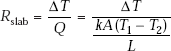
…from Eq. (2.7)
i.e.
Note: Many times, weight of insulation may be a criterion while selecting insulation. In such cases, we have,
i.e. for a specified thermal resistance, material with smallest product of r and k will be the lightest. The analysis shown above to determine the temperature profile and heat flux is the standard approach to solve a heat conduction problem, i.e. write down the general differential equation in the appropriate coordinate system, simplify it with the assumptions applicable to the problem at hand and then solve it in conjunction with the boundary conditions to get the temperature distribution; once the temperature distribution is known, heat flux is calculated by the application of Fourier’s law.
Alternatively:
For steady state heat conduction with no heat generation, let us apply the First law, namely,
Since there is no heat generation, Egen = 0 and RHS = 0 since it is steady state.
i.e.
This means that energy entering the system (i.e. slab, in this case) is equal to the energy leaving the system, i.e. Q is a constant. Then, we can directly integrate the Fourier’s equation. Even though Q is not known to start with, we know that it is a constant and therefore, Q can be taken out of the integral sign. We proceed as follows: Refer to Fig. 4.1. From Fourier’s law, we have,
Separating the variables and integrating from x = 0 to x = L (with T = T1 to T = T2), we get,
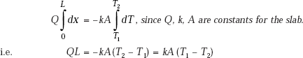
i.e.
Note that Eq. 4.12 for heat transfer rate is the same as Eq. 4.7.
To get temperature distribution: Integrating Eq. 4.11 between x = 0 and x = x. (with correspondingly, T = T1 and T = T (x)), we get,
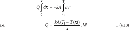
Now, remember that in steady state, Q is the same through each layer of the slab. So, equating Eqs. 4.12 and 4.13, we get,
i.e.
i.e.
Note that Eq. 4.14 is the same as Eq. (4.4). From Eq. 4.14, we can write the temperature distribution in the slab in non-dimensional form as follows,
Note that Eq. 4.15 is the same as Eq. 4.5
Note: Above alternative analysis is applicable only for steady state conduction, with no internal heat generation.
4.3 Heat Transfer through Composite Slabs
Heat transfer through a composite slab, consisting of 2 or 3 layers of materials of different thermal conductivities, is considered next. This is a very common application, e.g. in the case of insulation of furnace walls, insulation of walls of buildings, refrigerators, cold storage plants, hot water tanks, etc.
While solving heat transfer problems in composite slabs under steady state conditions, it is convenient to use the thermal resistance concept.
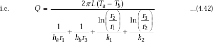
Consider a composite slab consisting of three layers 1, 2 and 3 as shown in Fig. 4.2. Let the thicknesses of the three layers be L1, L2 and L3, respectively; also, the respective thermal conductivities are k1, k2 and k3.
On the LHS of the composite slab, a fluid at a temperature Ta flows on the surface with a convective heat transfer coefficient of ha and on the RHS of the slab, a fluid at a temperature of Tb flows with a convective heat transfer coefficient of hb, as shown. Let Ta be higher than Tb, so that steady state heat transfer rate Q is from left to right as indicated in the Fig. 4.2.
Assumptions:
- Steady state, one-dimensional heat conduction.
- No internal heat generation.
- Constant thermal conductivities k1, k2 and k3.
- There is perfect thermal contact between layers, i.e. there is no temperature drop at the interface and the temperature profile is continuous.
Since it is a case of steady state conduction with no internal heat generation, it is clear from the First law that heat flow rate Q, through each layer is the same. Referring to Fig. 4.2, it may be seen that heat flows from the fluid at temperature Ta to the left surface of slab 1 by convection, then by conduction through slabs 1, 2 and 3, and then, by convection from the right surface of slab 3 to the fluid at temperature Tb.
Let the area of the slab normal to the heat flow direction be A (m2). Now, considering each case by turn,
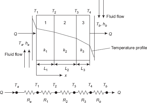
FIGURE 4.2 Composite slab with three layers and the thermal resistance network
Convection at the left surface of slab 1
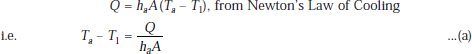
Conduction through slab 1
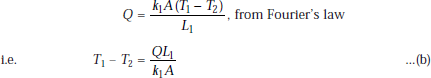
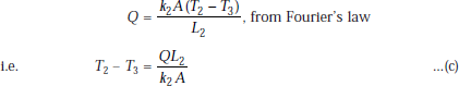
Conduction through slab 2
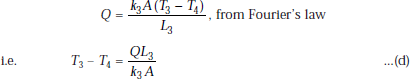
Conduction through slab 3
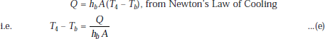
Convection at the right surface of slab 3
On adding Eqs. a, b, c, d and e, we get
i.e.
where, |
Ra = convective resistance at left surface of slab 1, |
|
R1 = conductive resistance of slab 1, |
|
R2 = conductive resistance of slab 2, |
|
R3 = conductive resistance of slab 3, and |
|
Rb = convective resistance at right surface of slab 3. |
So, we write Eq. g as:
Now, observe the analogy with Ohm’s law. Refer to the Fig. 4.2 for the equivalent thermal circuit. It is clear that (Ta – Tb) is the total temperature potential, Q is the heat current flowing and the total resistance is the sum of the individual five resistances which are in series.
For thermal resistances in series, we have,
For thermal resistances in parallel
Thermal resistances may be arranged in parallel too, as shown in Fig. 4.3.
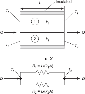
FIGURE 4.3 Composite slab with parallel resistances
Here, the main assumption is that the left hand and right hand faces of the composite slab are at uniform and isothermal temperatures T1 and T2, respectively, as shown in the Fig. 4.3. Also, the lateral surfaces are insulated so that the heat flow can be considered as one-dimensional, in the X-direction only.
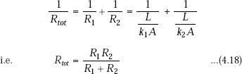
From the analogy with the electrical circuit, when the resistances are in parallel, the total resistance is given by:
For thermal resistances in series and parallel: General case of thermal resistances arranged in series and parallel is shown in Fig. 4.4.
Again, remember that one-dimensional heat flow is assumed; strictly, this is possible only when all the materials of the composite slab have the same value of thermal conductivity. If the thermal conductivities of materials 1, 2 and 3 differ greatly, then obviously, the heat flow will not be one-dimensional since the heat will tend to flow through the path of least resistance. Therefore, it is necessary that for practical purposes, for one-dimensional flow to be applicable, the thermal conductivities do not vary drastically.
Applying the rules of electrical circuit for series and parallel resistances, we have,
where, Reff is the effective resistance of the three resistances R2, R3 and R4 in parallel, as shown in Fig. 4.5.
i.e.
Note: Observe that the concept of thermal resistance is very useful in solving heat transfer problems in multiple layers of different thermal conductivities and also when multimodes of heat transfer are present. Only conditions to be satisfied to apply this concept are (i) steady state heat transfer, and (ii) no internal heat generation.
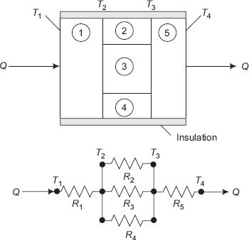
FIGURE 4.4 Composite slab with series–parallel resistances and the equivalent thermal circuit
4.4 Overall Heat Transfer Coefficient, U (W/(m2C))
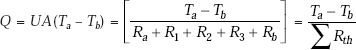
Consider the case of a furnace where heat is transferred by the hot gases to the inside surface by convection, then by conduction through one, two or three layers of brick and insulation, and finally to ambient air by convection at the outermost surface. This situation is represented in Fig. 4.2.
Now, in most of the practical cases, temperature of the hot gases (Ta) and that of the ambient (Tb) are known; intermediate temperatures are not known. We would like to have the heat transfer given by a simple relation of the form
where, Q is the heat transfer rate (W), A is the area of heat transfer perpendicular to the direction of heat transfer, and (Ta – Tb) = ΔT is the overall temperature difference.
Our problem is to derive a relation for U.
Now, we have from Eq. 4.16,
Comparing Eq. 4.16 and Eq. 4.21, we can write
i.e.
i.e.
Or,
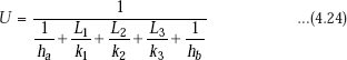
Remember the expression for U as given by Eq. 4.23; it is easier and is applicable when we deal with other geometries, too.
Concept of overall heat transfer coefficient is particularly useful in heat exchanger designs. Consider a heat exchanger where a hot fluid flows on one side of a heat exchanger wall and a cold fluid flows on the other side. Then, heat transfer is by convection on the hot side, by conduction across the separating wall and again by convection on the cold side. In such a case, overall heat transfer coefficient is obtained by applying Eq. 4.23. Values of overall heat transfer coefficients for many practical cases are tabulated in handbooks (see the chapter on heat exchangers).
Example 4.1. Determine the steady state heat transfer through a double pane window, 0.8 m high, 1.5 m wide, consisting of two 4 mm thick glass layers (k = 0.78 W/(mC)), separated by a 10 mm thick stagnant layer of air (k = 0.026 W/(mC)). Inside temperature of room air is maintained at 20°C with a convective heat transfer coefficient of ha = 10 W/(m2C). Outside air temperature is –10°C and the convective heat transfer coefficient on the outside is hb = 40 W/(m2C). Also, determine the overall heat transfer coefficient.
Solution. The schematic diagram and the equivalent thermal circuit is shown in Fig. Example. 4.1.
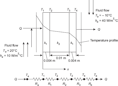
FIGURE Example 4.1 Double pane window and equivalent thermal circuit
This is the case of steady state, one-dimensional conduction, without internal heat generation, through a composite slab. Therefore, we can conveniently apply the thermal resistance concept. Note that heat transfer occurs from left to right, i.e. from the warm, inside air to the glass surface on the left by convection, then by conduction through the glass layer, then again by conduction through the stagnant air layer (no convection here since the air layer is stagnant), and by conduction through the second glass layer and finally, by convection to the outside cold air.
Let us solve this problem in Mathcad:
Data:
L1 := 0.004 m, L2 := 0.01 m, L3 := 0.004 m, Ta := 20°C Tb := 10°C ha := 10 W/(m2C) hb :=40 W/(m2C) k1 := 0.78 W/(mC) k2 := 0.026 W/(mC) k3 := k1 W/(mC) A := 1.5 × 0.8 m2 i.e. A = 1.2 m2
Convective resistance on the inside, Ra:
Conductive resistance through first glass layer, R1:
Conductive resistance through stagment air layer, R2:
Conductive resistance through second glass layer, R3:
Convective resistance on the outside, Rb:
Since all the resistances are in series, we write,
|
Rtot := Ra + R1 + R2 + R3 + Rb |
i.e. |
Rtot = 0.433 C/W … total themal resistance |
Therefore, heat transfer rate through the double pane window is given by,
|
|
i.e. |
Q = 69.248 W |
Overall heat transfer coefficient, U:
|
|
|
i.e. |
U = 1.924 W/(m2C). |
|
Note the magnitudes the thermal resistances offered by the glass layer and the air layer. Resistance of air layer is much more because of its poor thermal conductivity.
It is instructive to see what will be the heat flow rate if a window with a single glass layer is used. In such a case,
If a single layer glass window is used:
Observe the difference in heat flow rates for a single glass window and a double pane window. This is the reason why double pane windows are used, particularly in cold weather. Of course, an additional advantage is that it shields the residents from outside noise, too.
Example 4.2. Find the heat flow rate through the composite wall shown below, in Fig. 4.7. Assume one-dimensional conduction. Thermal conductivities of slabs A, B, C and D are 150, 30, 65 and 50 W/(mC), respectively. (M.U. Dec. 1997)
Solution. This is a case of steady state, one-dimensional heat conduction in composite slabs with no internal heat generation. Therefore, thermal resistance concept may be used very conveniently.
Referring to the Fig. Ex. 4.2 we can write,
where, |
ΔT = Total temperature difference |
|
RA = thermal resistance of slab A |
|
RBC = effective thermal resistance of slabs B and C, which are in parallel |
|
RD = thermal resistance of slab D. |
Calculations are done using Mathcad:
Data:
AA:= 100 × 10−4 m2 AB := 30 × 10−4 m2 AC := 70 × 10−4 m2 AD := 100 × 10−4 m2 LA := 0.03 m LB := 0.08 m LC := 0.08 m LD := 0.05 m kA := 150 W/(mC) kB := 30 W/(mC) kC := 65 W/(mC) kD:= 50 W/(mC) DT := (400 − 60) deg.C
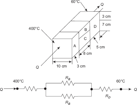
FIGURE Example 4.2 Composite slab with series–parallel resistances
Calculate the thermal resistances:
|
|
|
|
|
|
|
|
Now, resistances RB and RC are in parallel; Let their effective resistance be RBC:
Then, ![]() i.e. RBC = 0.147 C/W
i.e. RBC = 0.147 C/W
Total thermal resistance: |
Rtot := RA + RBC + RD |
Adding: |
Rtot = 0.267 C/W |
|
|
i.e. |
Q = 1.274 × 10³ W. |
Example 4.3. A composite wall consists of a 10 cm layer of building brick (k = 0.7 W/(mC)) and 3 cm thick plaster (k = 0.5 W/(mC)). An insulation material of k = 0.08 W/(mC) is to be added to reduce the heat transfer through the wall by 70%. Determine the thickness of the insulating layer.
Solution. In this case the temperatures on either side of the composite wall are not given. So, we assume that the overall temperature difference ΔT remains the same in both the cases. Also, since it is the case of steady state heat transfer with no internal heat generation, we can apply the thermal resistance concept. We have:
Case (i): steady state heat transfer for the composite wall consisting of building brick and plaster. Let the steady state heat transfer rate be Q; let the thermal resistances of the building brick be R1 and that of plaster be R2.
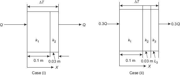
FIGURE Example 4.3 Composite wall without and with insulation
Case (ii): steady state heat transfer for the composite wall consisting of building brick and plaster plus the insulation layer. Now, from problem statement, the steady state heat transfer rate will be 0.3 Q; thermal resistances of the building brick, plaster and insulation are R1, R2 and R3, respectively.
These two cases are depicted in Fig. Example 4.3.
We have, for case (i): Q = ΔT/(R1 + R2), and
for case (ii): 0.3 Q = ΔT/(R1 + R2 + R3)
Dividing: (R1 + R2)/(R1 + R2 + R3) = 0.3
Considering a heat transfer area of A = 1 m2, let us do the calculations in Mathcad:
Data:
L1 := 0.1 m L2 := 0.03 m k1 := 0.7 W/(mC) k2 := 0.5 W/(mC) k3 := 0.08 W/(mC) A := 1 m2 L3, thickness of insulation layer is to be found out
Thermal resistances:
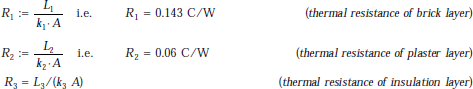
Therefore, R1 + R2 = 0.203 C/W
And, (R1 + R2)/(R1 + R2 + R3) = 0.3
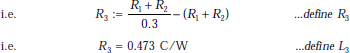
Therefore, thickness of insulation layer:
|
L3 := R3·k3·A |
|
i.e. |
L3 = 0.038 m |
(thickness of insulation layer required to reduce the heat transfer rate by 70%) |
Example 4.4. A square plate heater (size: 15 cm × 15 cm) is inserted between two slabs. Slab A is 2 cm thick (k = 50 W/ (mK)) and slab B is 1 cm thick (k = 0.2 W/(mK)). The outside heat transfer coefficients on both sides of A and B are 200 and 50 W/(m2K), respectively. Temperature of surrounding air is 25°C. If the rating of heater is 1 kW, find:
- maximum temperature in the system
- outer surface temperatures of two slabs.
Draw the equivalent circuit for the system (P.U. Nov. 1994)
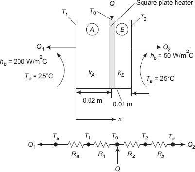
FIGURE Example 4.4 Two slabs with a plate heater in between and the thermal circuit
Solution. This is a case of steady state conduction, with no internal heat generation within the slabs. So, thermal resistance concept can be applied. Note that, obviously, the maximum temperature, T0, will occur at the heater in between the slabs; and, the total heat supplied, Q, is divided into two portions: Q1 flowing out to the left and Q2 flowing out to the right, as shown in Fig. Example. 4.4.
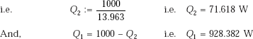
We use the condition: Q = Q1 + Q2 = 1000 W
Consider one m2 area of heat transfer, i.e. A = 1 m2
Then, |
Q1 = (T0 – Ta)/(R1 + Ra), and |
|
Q2 = (T0 – Ta)/(R2 + Rb) |
where, |
R1 = thermal resistance of slab A |
|
R2 = thermal resistance of slab B |
|
Ra = convective resistance on the left face of A, and |
|
Rb = convective resistance on the right face of slab B. |
Let us get the solution in Mathcad:
Data:
LA := 0.02 m LB := 0.01 m kA := 50 W/(mK) kB := 0.2 W/(mK) ha := 200 W/(m2K) hb := 50 W/(m2K) Ta := 25°C A := 0.15·0.15 m2
i.e. A = 0.022 m2 Q := 1000 W (rating of the heater)
Let the temperature at the heater be T0…to be found out
Thermal resistances:
|
|
|
|
|
|
|
|
|
|
|
|
To get Q1 and Q2, We have,
i.e.
and,
Solve Eqs. a and b simultaneously to get Q1 and Q2:
Therefore, Q1 = 12.963 Q2
Now, since Q1 + Q2 = 1000, we get
|
12.963 Q2 + Q2 = 1000 |
i.e. |
13.963 Q2 = 1000 |
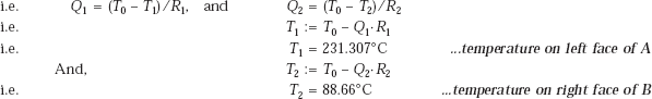
To calculate maximum temperature, T0, We have
Therefore:
T0 := Q1·(R1 + Ra) + Ta |
i.e. T0 = 247.812°C |
…maximum temperature in the system |
Verify:
|
|
|
To get T1 and T2, we calculate T1 and T2 applying the Fourier’s law to slab A and B separately:
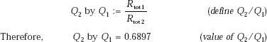
Example 4.5. A composite insulating wall has three layers of material held together by 3 cm diameter aluminium rivet per 0.1 m2 of surface. The layers of material consist of 10 cm thick brick, with hot surface at 200°C, 1 cm thick wood with cold surface at 10°C. These two layers are interposed with a third layer of insulation material 25 mm thick. Thermal conductivities of materials are: k (brick) = 0.93 W/(mK), k (ins) = 0.12 W/(mK), k (wood) = 0.175 W/(mK) and k(Al) = 204 W/(mK). Assuming one dimensional heat flow, calculate the percentage increase in heat transfer rate due to rivets.
Solution. Consider 0.1 m2 area of the wall. By data, this area contains one alumilium rivet of 3 cm diameter.
Since this is a case of steady state conduction with no internal heat generation, we can apply the thermal resistance concept.
There are two cases of heat transfer, (a) with the rivet let the heat transfer rate be Q1, and (b) without the rivet let the heat transfer rate be Q2. Now, the total temperature drop is the same for both the cases, i.e (200 – 10) = 190 deg.C.
Therefore,
(Q2/Q1) = (Total thermal resistance with the rivet)/(Total thermal resistance without the rivet)
Mathcad solution to this problem is given below:
Data:
Lbrick := 0.1 m Lins := 0.025 m Lwood := 0.01 m d := 0.03 m L := Lbrick + Lins + Lwood
i.e. L = 0.135 m kbrick := 0.93 W/(mK) kins := 0.12 W/(mK) kwood := 0.175 W/(mK) kAl := 204 W/(mK) A := 0.1 m2
Area of rivet: ![]()
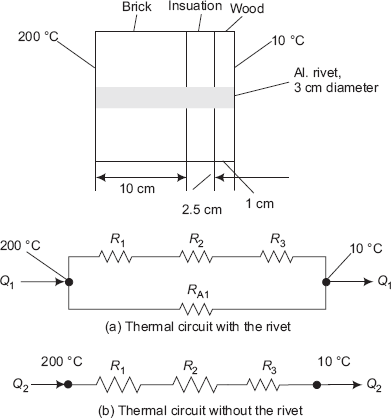
FIGURE Example 4.5 Composite slab with aluminium rivet
i.e. Arivet = 7.069 × 10⁻⁴ m2
Thermal resistances: Let the thermal resistances of brick, insulation and wood, without the rivet in position, be R1, R2 and R3, respectively. Then,
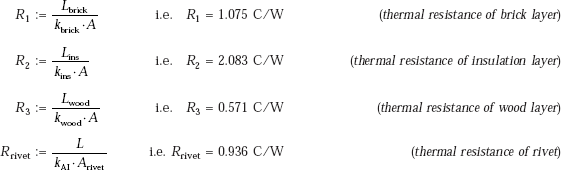
Now, without the rivet, total thermal resistance is = (R1 + R2 + R3), since all the resistances are in series.
When, the aluminium rivet is in place, strictly speaking, while calculating the thermal resistances of brick, insulation and wood, area used must be = (0.1 m2 minus the area of rivet); however, note that area of rivet is very small (i.e. 0.0007068 m2) compared to 0.1 m2. Therefore, with the rivet also, we use the same area of 0.1 m2, i.e. we use the same R1, R2 and R3.
Without the rivet, total thermal resistance, Rtot:
Rtot = R1 + R2 + R3, i.e. Rtot = 3.730031 C/W
With the rivet, total thermal resistance, Reff:
Now, refer to Fig. Example 4.5 Rtot is in parallel with Rrivet. Therefore,
Let Q1 = heat transfer rate with the rivet and Q2 = heat transfer rate without the rivet
Let Q2 by Q1 = Q2/Q1. Since temperature difference is same, i.e. (200 – 10) = 190°C in both cases,
Q2/Q1 is equal to the ratio, (Rwith rivet)/(Rwithout rivet)
![]() i.e. Q2 by Q1 = 0.201
i.e. Q2 by Q1 = 0.201
Therefore, % increase in heat transfer,
|
Increase = (Q1 − Q2) × 100/Q1 = [1 − (Q2/Q1)] × 100 |
|
|
Increase := (1 − Q2 by Q1) · 100 |
|
i.e. |
Increase = 79.937% |
(percentage increase in heat transfer rate due to aluminium rivet) |
Note: To be accurate, while calculating the thermal resistances of brick, insulation and wood, if we consider the area as 0.1 m2 minus the area of rivet, i.e. 0.0992932 m2 instead of 0.1 m2, we get the following results:
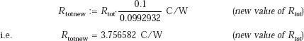
With the rivet in place:
Note that new value of Reff has become 0.749 as compared to earlier value of 0.748.
And, to calculate the increase in heat transfer,
|
Increase := (1 − Q2 by Q1) · 100 |
|
|
i.e. |
Increase = 80.05% |
(Note that this is not much different from earlier value of 79.937%.) |
|
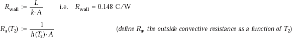
Example 4.6. The inside temperature of a furnace wall, 200 mm thick, is 1350°C. The mean thermal conductivity of wall material is 1.35 W/(mC). The heat transfer coefficient of outside surface is a function of temperaturte difference and is given by:
h = 7.85 + 0.08 × ΔT where ΔT is the temperature difference between outside wall surface and surroundings. Determine the rate of heat transfer per unit area, if the surrounding temperature is 40°C. (M.U., May 2000)
Solution. Refer to Figure Example 4.6.
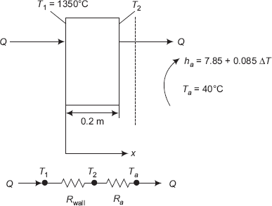
FIGURE Example 4.6 Furnace wall with convection on outside surface
Data:
A := 1 m2 T1 := 1350°C L := 0.2 m Ta := 40°C k := 1.35 W/mC h(T2) := 7.85 + 0.08·(T2 − Ta)
Since we have steady state heat transfer with no internal heat generation, we apply the thermal resistance concept. Also, the heat transfer rate, Q is the same through each layer, i.e. through the furnace wall as well as through the convective layer adjacent to the outside surface of the furnace wall.
Thermal resistances:
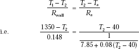
Now, the heat transfer rate through the wall is equal to the heat transfer rate through the outside convective layer.
i.e. |
Q = (T1 − T2)/Rwall, and |
|
Q = (T2 − Ta)/Ra |
When we equate these two equations and simplify, we get a quadratic equation in T2. Then solve it for T2. Once we get T2, we can easily calculate Q by applying any one of the above two equations.
We have:
Simplifying, we get,
This is a quadratic equation in T2, whose roots are given by,
where, a = 0.01184, b = 1.2146 and c = –1377.528
On substituting, the values of a, b and c, we get
Solving, we get
|
T2 = 293.637°C |
And |
Q = (1350 − 293.637)/0.148 |
|
= 7137.59 W. |
Note: The above procedure is, however, cumbersome. But, with Mathcad, the problem is easily solved using the solve block. Here, we start with a trial value of T2 and then, write the constraint, i.e. the equality of the above two equations, within the solve block, just after Given. Then, the command Find(T2) immediately gives the value of T2.
(Trial value)
Given
Find(T2) = 293.508
T2 := 293.508°C |
(temperature of outside surface of furnace wall) |
To find heat transfer rate, Q:
|
|
(the heat transfer rate per m2.) |
Verify:
Considering the convective layer:
|
|
|
Note: The values of Q obtained by the two methods are almost same, as it should be.
4.5 Thermal Contact Resistance
So far, while dealing with composite slabs, we assumed that there is perfect thermal contact at the interface, which means that there is no temperature drop at the interface. However, in many cases, particularly when the mating surfaces are rough, this may not be true and there will be a temperature drop at the interface. This temperature drop at the interface is due to what is known as contact resistance.
Physical reasoning for contact resistance is explained with reference to Fig. 4.5.
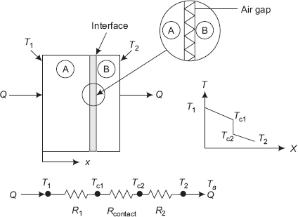
FIGURE 4.5 Thermal contact resistance
Figure. 4.5 shows an enlarged view of the interface between two slabs A and B. It may be observed that though the surfaces are smooth, physical contact between A and B occurs only at a few points, i.e. at the peaks as shown. Therefore, heat transfer occurs by conduction through this solid contact area and also by gas conduction through the gas filling the interfacial voids. Note that there is no convection in the interfacial gas since the space of interfacial voids is very small; Also, at the temperatures normally encountered, radiation is negligible. So, in effect, resistance to heat transfer is by two mechanisms:
- by solid conduction at the peaks, and
- by gas conduction through the interfacial gas in the voids.
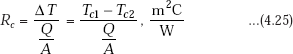
Of these two, solid conduction is usually negligible. Note that there is a temperature drop at the interface, (Tc1 − Tc2) and the temperature profile is not continuous. Thermal contact resistance is defined as the temperature drop at the interface divided by the heat transfer rate per unit area.
Interface thermal contact conductance is defined as the inverse of the contact resistance, and is given by:
Thermal contact resistance depends on:
- surface roughness—smoother the surface, lesser the resistance
- interface temperature—higher the temperature, lesser the resistance
- interface pressure—higher the pressure, lesser the resistance
- type of material—softer the material, lesser the resistance
Thermal contact resistance may be reduced by:
- making the mating surfaces very smooth
- inserting a layer of conducting grease (such as silicon based thermal grease, whose thermal conductivity is about 50 times that of air) at the interface
- inserting a ‘shim’ (thin foil) made of a soft material such as indium, lead, tin or silver between the surfaces
- filling the interstitial voids with a gas of higher thermal conductivity than that of air (e.g. helium)
- increasing the interface pressure
- in case of permanently bonded joints, contact resistance can be reduced by using an epoxy or soft solder rich in lead, or a hard solder of gold/tin alloy
Table 4.1 below gives thermal contact resistance for metallic interfaces under vacuum conditions, at different externally applied pressures.
Table 4.2 illustrates the effect of interfacial fluid on the thermal resistance, for the specific case of an aluminium interface, with the surfaces having 10 μm roughness and the pressure being 105 N/m2.
Thermal contact resistance of some typical solid/solid interfaces is given Table 4.3.
TABLE 4.1 Thermal contact resistance (Rc × 104, m2K/W), with vacuum at interface
| Contact pressure | 100 kN/m2 | 10,000 kN/m2 |
|---|---|---|
Stainless steel |
6 – 25 |
0.7 – 40 |
Copper |
1 – 10 |
0.1 – 0.5 |
Magnesium |
1.5 – 3.5 |
0.2 – 0.4 |
Aluminium |
1.5 – 5.0 |
0.2– 0.4 |
TABLE 4.2 Thermal contact resistance, Rc, for AI interface with surface roughness of 10 μm (Pressure = 105 N/m2)
| Interfacial fluid | Rc × 104, (m2K/W) |
|---|---|
Air |
2.75 |
Helium |
1.05 |
Hydrogen |
0.72 |
Silicon oil |
0.525 |
Glycerine |
0.265 |
TABLE 4.3 Thermal contact resistance, Rc, for some solid/solid interfaces
| Interface | Rc × 104, (m2K/W) |
|---|---|
Silicon chip/lapped Al in air (27 – 500 kN/m2) |
0.3 – 0.6 |
Al/Al with indium foil filter (~100 kN/m2) |
~0.07 |
S.S/S.S with indium foil filter (~3500 kN/m2) |
~0.04 |
Al/Al with Dow corning 340 grease (~100 kN/m2) |
~0.07 |
S.S/S.S with Dow corning 340 grease (~3500 kN/m2) |
~0.04 |
Silicon chip/Al with 0.02 mm epoxy |
0.2 – 0.9 |
Brass/Brass with 15 μm tin solder |
0.025 – 0.14 |
Values of Rc are given in heat transfer handbooks.
Generally, contact resistance is in series with other resistances and is taken into account by adding the same to other resistances. If the area of contact is given (= A) and Rc (in m2C/W) is known, then, Rc/A will give the contact resistance (in C/W) for the given area.
Following problem will clarify the use of this concept.
Example 4.7. Consider a plane composite wall that is composed of two materials of thermal conductivities kA = 0.1 W/ (mK) and kB = 0.04 W/(mK) and thicknesses LA = 10 mm and LB = 20 mm. The contact resistance at the interface between the two materials is known to be 0.3 m2K/W. Material A adjoins a fluid at 200°C for which h = 10 W (m2K) and material B adjoins a fluid for which h = 20 W/(m2K).
- What is the rate of heat transfer through a wall that is 2 m high and 2.5 m wide?
- Determine the overall heat transfer coefficient.
- Sketch the temperature distribution.
Solution. Refer to Fig. Example 4.7.
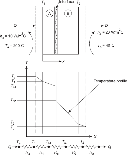
FIGURE Example 4.7 Two slabs with contact resistance at the interface
Data:
LA := 0.01 m LB := 0.02 m kA := 0.01 W/(mK) kB := 0.04 W/(mK) Ta := 200°C Tb := 40°C ha := 10 W/(m2K) hb := 20 W/(m2K) A := 2·2.5 m2 Rinterface := 0.3 (m2K)/W
Since it is steady state heat transfer and there is no internal heat generation, we can apply the thermal resistance concept. Overall temperature drop, i.e. the temperature potential, ΔT = (200 – 40) = 160 deg. C. And, the resistances involved are: two convective resistances, two conductive resistances of slabs A and B, and the contact thermal resistance at the interface. All these resistances may be calculated for a heat transfer area of 5 m2 and then added up together since all of them are in series. Then, rate of heat transfer is calculated as, Q = ΔT/Rtot
Thermal resistances:
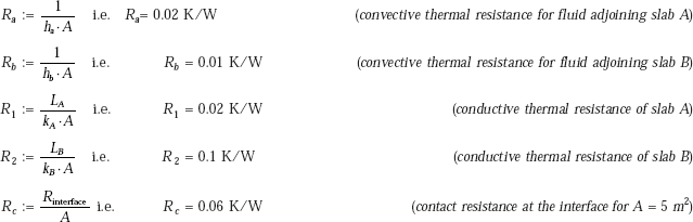
Therefore, total thermal resistance, Rtot:
Rtot := RA + R1 + Rc + R2 + Rb i.e. Rtot = 0.21 K/W
Heat transfer rate, Q:
|
|
|
Overall heat transfer coefficient, U:
|
|
i.e. |
U = 0.952 W/(m2K) |
Temperature drops:
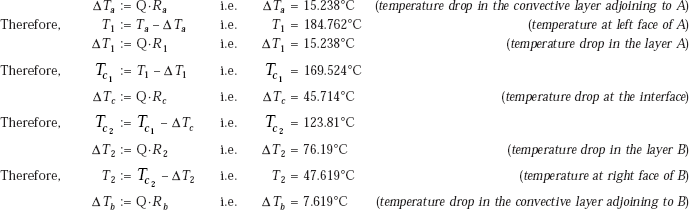
Check: the temperature Tb must equal 40°C
4.6 Conduction with Variable Area
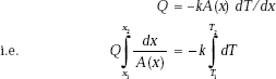
While considering Fourier’s law, namely,
the area A is normal to the direction of heat transfer. In case of plane slabs studied so far, the area normal to the direction of heat flow was constant. However, this need not be the case always. In practice, many times, we come across solid shapes like truncated cones, truncated wedges, developed cylinder, etc. that may be used as structural members, struts or supports. Analysis of heat transfer through such members is easily done by direct integration of Fourier’s equation, under the following conditions:
- One-dimensional conduction
- Steady state heat transfer
- No internal heat generation
- Variation of area can be expressed mathematically as a function of x.
Consider a truncated cone as shown in Fig. 4.6.
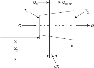
FIGURE 4.6 Conduction through variable area
The left face of the truncated solid is at the coordinate position x1 and the right face is at coordinate position x2, as shown. Let the left face be at temperature T1 and the right face at T2. Let T1 > T2. We would like to find out the heat transfer rate Q and the temperature distribution in the solid, under steady state corditions.
Consider a differential control volume between x = x and x = x + dx.
By applying the First law, it is clear that heat transfer rate, Qx = Qx + dx, since there is steady state, one-dimensional heat transfer with no internal heat generation, i.e. the heat transfer rate is the same through all sections and is a constant, Q. Further, let us say that area A is a function of x and can be expressed mathematically as A = A (x).
To start with, we do not know the value of Q, but we do know that it is a constant; so, we can take Q out of the integral sign, while directly integrating Fourier’s equation,
for the general case when thermal conductivity, k, is a function of temperature, T.
Separating the variables,
Now, integrating between x = x1 and x = x2, with corresponding T = T1 and T = T2,
we write,
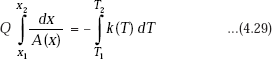
If k is a constant and does not vary with temperature, we can write,
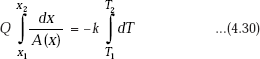
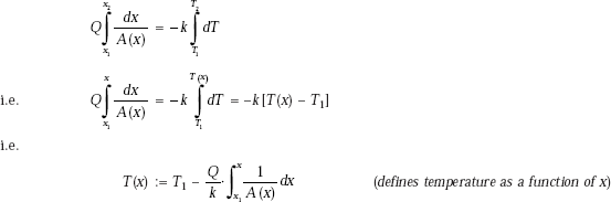
Now, if T1 and T2 at any two corresponding x values of x1 and x2 are known, then Q can be calculated from the Eq. 4.30. To obtain the temperature distribution in the solid, we use the condition that Q is the same through each layer in steady state, i.e. get Qx by integrating between x1 and any x (i.e. temperature varying from T1 to T(x)) and equate this to the already obtained value of Q.
If k is varying with temperature, use Eq. 4.29 and follow the same procedure.
We illustrate the method by solving a problem.
Example 4.8. A conical cylinder of length L and radii R1 and R2, (R1 < R2) is fully insulated on the outer surface. The two ends are maintained at T1 and T2, (T1 > T1). Considering one-dimensional steady state heat flow, derive expressions for heat flow and temperature distribution.
As a numerical example, taking: R1 = 1.25 cm, R2 = 2.5 cm, L = 20 cm, T1 = 227°C, T2 = 27°C, k = 40 W/(mC), find:
- steady state heat transfer rate, Q
- temperature at mid-plane
- temperature at a plane 15 cm from the small end
- draw the temperature profile in the solid
Solution. Refer to Fig. Example 4.8.
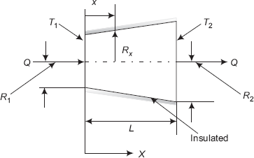
FIGURE Example 4.8 Conduction with variable area
Assumptions:
- steady state
- one-dimensional conduction, in X-direction (since sides are insulated)
- no internal heat generation
- constant k
To determine heat transfer rate:
At any distance x from the origin, heat transfer rate Qx is given by:
where, Ax is the area normal to the direction of heat flow at x.
Radius at x is given by:
where ![]()
Now,
Therefore,
Separating the variables and integrating from x = 0 to x = L and correspondingly, T = T1 to T = T2, we get:
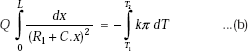
Note that Q is taken out of the integral sign since it is a constant and is the same at all sections.
Now, LHS of Eq. b is given by:
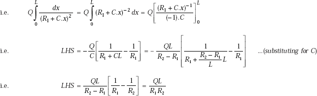
since, C = (R2 − R1)/L
RHS of Eq. b is given by:
On equating LHS and RHS, we get
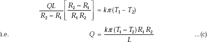
Eq. c is the desired expression for the heat transfer rate.
To determine temperature distribution:
Let temperature at any x be T(x).
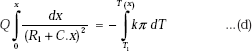
General procedure is to equate the expression for heat transfer at any x obtained by integrating Eq. b between x = 0 and x = x (i.e. between T = T1 and T = T(x)), and the expression c derived above for Q between the two sections at known temperatures of T1 and T2.
So, Eq. b becomes:
Now, LHS of Eq. d becomes:
Remembering that C = (R2 – R1)/L and Rx = R1 + C.x, we get:
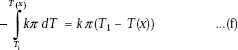
RHS of Eq. d becomes:
Now, equate the two expressions for Q, given by Eqs. c and g,
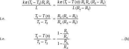
Eq. h gives the expression for temperature distribution in the solid as a function of x. Again, remember that Rx is the radius at any x and is given by:
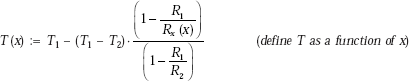
Now, let us solve the numerical example in Mathcad. Refer to Fig. Example 4.8.
Data:
R1 := 0.0125 m R2 := 0.025 m T1 := 227°C T2 := 27°C L := 0.2 m k := 40 W/(mC)
Heat transfer rate, Q:
On substituting values, we get
Q = 39.27 W (heat transfer rate through the section)
Tempearature at mid-plane, i.e. at x = 0.1 m:
x := 0.1 m (at mid-plane of the section)
We have, at x = 0.1 m, Rx = R1 + (R2 − R1).(x/L)
Therefore:
i.e. Rx(0.1) = 0.1 m (radius at x = 0.1 m)
Now, temperature distribution is given by Eq. h derived above:
From Eq. (h):
Therefore,
T(0.1) = 93.667°C (temperature at mid-plane.)
Temperature at x = 15 cm from LHS:
Simply substitute x = 0.15 in T(x):
T(0.15) = 55.571°C (temperature at a plane 15 cm from LHS)
To draw the temperature profile within the solid:
In Mathcad, this is very easy. Define a range variable x, varying from x = 0 to x = 0.2 m. Temperature T(x) as a function of x is already defined. From the graph pallette, choose x – y graph and fill in the place holders on the x-axis and y-axis. Click anywhere outside the graph region and immediately the graph appears: (see Fig. Ex. 4.8(b) below)
x := 0.0.01, … , 0.2 (define the range variable x, varying from 0 to 0.2 m, at an interval of 0.01 m)
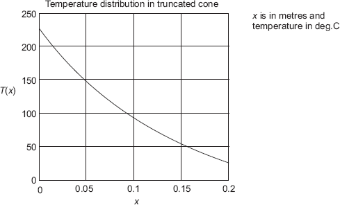
FIGURE Example 4.8(b)
Note from the graph that temperature at the mid-plane, i.e. at x = 0.1 m is 93.67°C, as calculated earlier.
Exercise: If the RHS, i.e. the larger diameter end, is at 227°C and the LHS is at 27°C, how does the heat transfer and the temperature distribution change?
Example 4.9. A structural support has the shape of a truncated cone (see Fig. Example 4.9) of length 0.2 m and its area varies with x as A = (π / 4).x3. Its circumference is perfectly insulated. Thermal conductivity of the material varies with temperature and is given by: k(T) = 14.695(1 + 0.0010208 T), where T is in deg. C and k is in W/(mC). What is the steady state heat transfer rate through this strut if the two ends are maintained at 400°C and 150°C, as shown? Also, find the temperature at the mid-plane. Draw the temperature profile in the solid.
Solution.
Data: ![]()
k(T) := 14.695(1 + 0.0010208T) W/(mC) T1 := 400°C T2 := 150°C
FIGURE Example 4.9 Conduction with variable area and variable thermal conductivity
Assumptions:
- steady state conduction
- one-dimensional conduction
- no internal heat generation
- k varying with temperature.
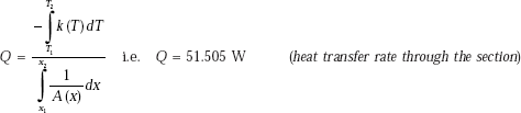
To find heat transfer rate, Q:
Since this is a case of steady state, one-dimensional conduction, with no internal heat generation, Q is constant through each section in the solid; so, we can directly integrate Fourier’s equation, keeping the Q outside the integral. Integrating between two known temperatures at x = x1 and x = x2, we calculate Q.
Substituting for k(T) and A(x):
Since Q is constant, separating the variables and integrating between x = 0.08 and x = 0.28 (with T1 = 400°C and T2 = 150°C), we get:
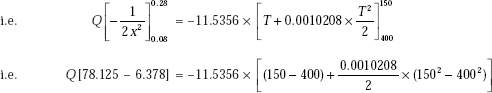
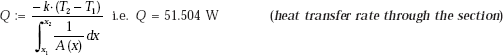
On simplifying, we get
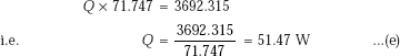
i.e. the steady state heat transfer rate for the solid is 51.47 W.
In Mathcad, above calculation is done just in one step; there is no need to expand the integral and substitute the values. We write directly from Eq. a:
This value of Q matches with the value obtained earlier.
To find temperature at mid-plane, i.e. at x = 0.18 m:
Let the temperature at mid-plane be Tm. Since, Q is a constant, which is already calculated, integrate between x = 0.08 and x = 0.18 with corresponding T = 400°C and T = Tm; we get a quadratic equation in Tm and solving it, get Tm:
Integrating Eq. c between x = 0.08 and x = 0.18, with T = 400°C and T = Tm, we get,
i.e.
On simplifying, we get,
Eq. g is a quadratic in Tm and its roots are given by,
where, a = 58.878 × 10⁻⁴, b = 11.5356 and c = – 2329.48
Substituting:
On solving, we get,
i.e. temperature at the mid-plane is 184.599°C.
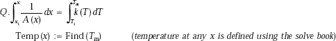
Above calculation is rather laborious to perform by hand. In Mathcad, it solved very easily using the solve block:
Temperature at the mid-plane, i.e. at x = 0.18 m:
Let the temperature at mid-plane (x = 0.18 m) be Tm. Integrate between x = 0.08 m and x = 0.18 m and use the condition that heat flow rate is the same (already calculated) through all sections. Use the solve block starting with a trial value of Tm:
x := 0.18 m |
(at mid-plane) |
Tm := 250°C |
(trial value of Tm) |
Given
Note that instead of just finding Tm by typing Tm =, we have defined it as equal to a function Temp (x) within the solve block. Advantage of doing this is that the same solve block repeatedly does the calculations for all values of x as desired, taking each time the starting trial value of temperature as 250. This facility is a great advantage and is used below while drawing the temperature profile.
Therefore, |
Temp(0.18) = 184.514 |
(temperature at x = 0.18 m) |
i.e. |
Tm = 184.514°C |
(temperature at mid-plane) |
Verify temperature at x = 0.08 m and x = 0.28 m:
Note that the mid-plane temperature obtained now matches the value obtained earlier.
To draw the temperature profile:
Define the range variable x from 0.08 m to 0.28 m at an interval of 0.01 m. Then, choose the x – y plot from the graph palette and fill in the place holders on the x-axis and y-axis. Click anywhere outside the graph region and the graph appears immediately: See Fig. Ex. 4.9(b)
x := 0.08, 0.09, …, 0.28 |
(define range variable x, varying from 0.08 m to 0.28 m, at interval of 0.01 m) |
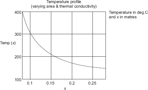
FIGURE Ex. 4.9(b)
Note: Verify from the graph that the temperature at the two ends and the mid-plane match with the values obtained earlier.
Also, observe the ease with which the temperature profile is drawn—calculation of temperature at each value of x and drawing the graph is done in one step; if this has to be done in hand calculation, to determine T at each x, one will have to solve a quadratic equation for T at each point. Obviously, it is a very tedious job.
If k is a constant, how does heat transfer and temperature distribution change?
Let k = 18.82 W/(mC)
Again, since Q is constant through each section in the solid, we can directly integrate Fourier’s equation, keeping the Q outside the integral. Integrating between two known temperatures at x = x1 and x = x2, we calculate Q.
In Mathcad, this is solved very easily:
From the above equation, we write for Q:
Note that this value of Q is the same as obtained earlier with variable k.
Temperature profile:
Let the temperature at any x be T(x). Integrate between x = 0.08 m and x = x and use the condition that heat flow rate is same (already calculated) through all sections.
We have:
Temperature at mid-plane:
Put x = 0.18 m in T(x):
Note that with constant k, the mid-plane temperature is 181.55°C whereas with variable k, it was 184.514°C.
To draw the temperature profile:
Define the range variable x from 0.08 m to 0.28 m at an interval of 0.01 m. Then, choose the x – y plot from the graph palette; type x in the place holder on the x-axis and Temp(x), T(x) in the place holder on the y-axis. Click anywhere outside the graph region; graphs for temperature distribution with variable k as well as with constant k, appear immediately: See Fig. Ex. 4.9(c)
x := 0.08, 0.09, …, 0.28 |
(define range variable x, varying from 0.08 m to 0.28 m, at an interval of 0.01 m) |
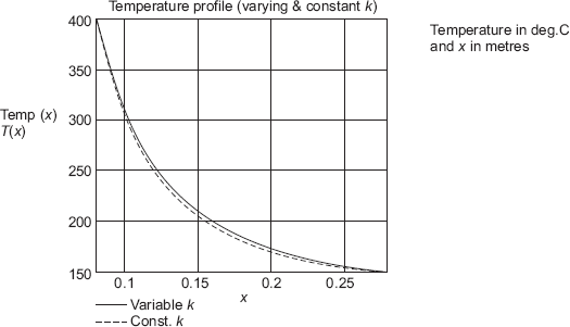
FIGURE Ex. 4.9(c)
It may be observed from the graph that with constant k assumption, temperature is lower throughout, as compared to the case of variable k.
4.7 Cylindrical Systems
Cylindrical systems are practically important because of their common application in varied industries, power plants, refineries, etc. Cylindrical geometry is popular for applications in heat exchangers, condensers, storage tanks, etc.
Here, we analyse the cylindrical shell for heat transfer in one-dimensional conduction, i.e. it is assumed that temperature gradients are significant only in the radial direction; so, heat flow occurs only in the radial direction. Now, it is important to remember that for a cylindrical system with heat flow in the radial direction, the area normal to the direction of heat flow is not a constant, but varies with r; this was not the case for a plane slab, where A remained constant for all x.
Consider a long cylinder of length L, inside radius ri and outside radius ro. Inner and outer surfaces are at uniform temperatures of Ti and To, respectively, see Fig. 4.7.
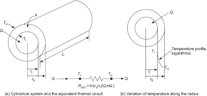
FIGURE 4.7 Heat transfer through a cylindrical shell
Assumptions:
- Steady state conduction
- One-dimensional conduction, in the r direction only
- Homogeneous, isotropic material with constant k
- No internal heat generation.
Now, this is a cylindrical system; so, it is logical that we start with the general differential equation for one-dimensional conduction, in cylindrical coordinates. So, we have, from Eq. 3.17:
In this case:
∂T/∂τ |
= |
0, since it is steady state conduction |
∂T/∂ϕ |
= |
0 = ∂T/∂z, since it is one-dimensional conduction, in the r direction only |
qg/k |
= |
0, since there is no internal heat generation. |
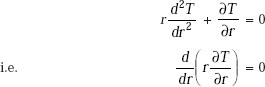
Therefore, the controlling differential equation for the cylindrical system, under the above mentioned stipulations, becomes:
Note that now, it is not partial derivative, since there is only one variable, r.
We have to solve this differential equation to get the temperature distribution along r and then apply Fourier’s law to calculate the heat flux at any position.
Multiplying Eq. 4.31 by r, we get
Integrating,
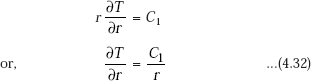
Integrating again,
where, C1 and C2 are constants of integration.
Eq. 4.33 gives the temperature distribution as a function of radius.
C1 and C2 are found out by applying the two B.C.’s:
- at r = ri, T = Ti
- at r = ro, T = To
B.C. (i) gives, |
Ti = C1 ln (ri) + C2 |
…(a) |
B.C. (ii) gives, |
To = C1 ln(ro) + C2 |
…(b) |
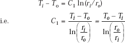
and, from Eq. a:
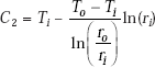
Substituting C1 and C2 in Eq. 4.33, we get
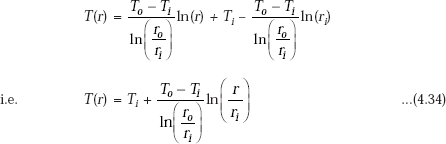
Eq. 4.34 is the desired equation for temperature distribution along the radius. Note that the temperature distribution is logarithmic for the cylindrical system, whereas it was linear for a plane slab. Temperature distribution for the cylindrical system is sketched in Fig. 4.7(b).
Eq. 4.34 is written in non-dimensional form as follows:
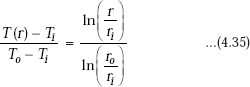
For thin cylinders, ri ≈ ro, and then the temperature distribution within the shell is almost linear.
Next, to find the heat transfer rate, Q:
We apply the Fourier’s law.
Considering the inner radius ri,
(using Eq. (4.32))
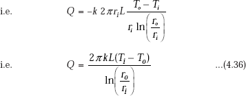
Eq. 4.36 gives the desired expression for rate of heat transfer through the cylindrical system.
Note that Q is dependent on ln(ro/ri) rather than on (ro – ri). Implication of this is as follows:
For the same ΔT, k and L, heat transfer rate through a cylindrical shell of 5 cm ID and 10 cm OD is the same as that through a shell of 10 cm ID and 20 cm OD, though in the first case, shell thickness is 5 cm and in the second case, the shell thickness is 10 cm.
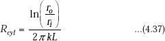
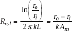
Now, writing Eq. 4.36 in a form analogous to Ohm’s law:
Immediately, we observe that thermal resistance for conduction for a cylindrical shell is given by,
Alternatively
For steady state, one-dimensional conduction, with no heat generation, since the heat flow rate is the same and constant at every crosssection, we can directly integrate the Fourier’s equation between the two known temperatures (and the corresponding, known radii), keeping Q out of the integral sign; this will give us Q. Then, at any r, the temperature T(r) is calculated by integrating between r = ri and r = r (with T = Ti and T = T(r)), and equating the Q obtained now to the expression for Q obtained earlier. Refer to Fig. 4.8.
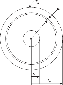
FIGURE 4.8 Cylindrical system
At any radius r, consider a thin cylindrical shell of thickness dr ; let the temperature differential across this thin layer be dT. Then, in steady state, rate of heat transfer through this layer Q, can be written from Fourier’s law, to be equal to:
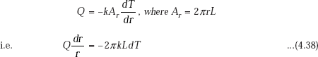
Integrating Eq. 4.38 from ri to ro (with temperature from Ti to To),
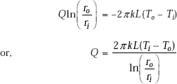
(same as Eq. 4.36)
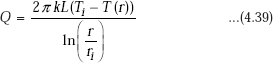
To get the temperature profile within the cylindrical shell:
At any radius r, let the temperature be T(r).
Integrating Eq. 4.38 from ri to r,
Now, apply the principle that in steady state, Q is the same through each layer, i.e. equate Eqs. 4.36 and 4.39:
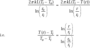
…same as Eq. 4.35
Concept of log mean area. For a plane slab, we have the simple relation for the thermal resistance, i.e. Rslab = L/(kA), where L is the thickness of the slab, k is the thermal conductivity and A is the cross-sectional area normal to the direction of heat flow.
Now, many times, it is desirable to write the thermal resistance of the cylindrical system also in a form analogous to this form of Rslab. Then, we take L as equivalent to (ro – ri), and k is the thermal conductivity, and let Am be an equivalent area of the cylindrical system, which is to be found out. Then, we write:
Therefore,
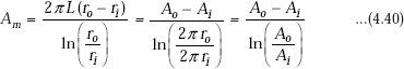
where, |
Ao = 2πro = outside surface area of the cylindrical shell |
|
Ai = 2 πri = inside surface area of the cylindrical shell |
|
Am is known as the log mean area for the cylindrical system. |
Note that physically, Am is the area of an equivalent slab having the same thermal conductivity k, whose thickness is equal to the thickness of the cylindrical shell, and has the same heat flow rate as for the cylindrical shell.
In practice, concept of log mean area is useful in analysing the lagging (i.e. insulation) of steam pipes.
If (Ao/Ai) < 2, then Am can be approximated to be the arithmetic average of Ao and Ai
i.e. Am = (Ao+ Ai)/2
Example 4.10. A cylindrical insulation for a steam pipe has an inside radius ri = 6 cm, outside radius ro = 8 cm and k = 0.5 W/(mC). The inside surface of the insulation is at a temperature Ti = 430°C and the outside surface is at To = 30°C. Determine:
- heat loss per metre length of this insulation
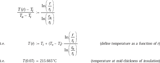
- temperature at mid-thickness of the insulation, and
- draw the temperature profile along the radius.
Solution. Data:
ri := 0.06 m ro := 0.08 m L := 1 m Ti := 430°C To := 30°C k := 0.5 W/(mC)
Heat transfer rate, Q:
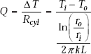
Since it is a case of steady state, one-dimensional conduction, with no internal heat generation, we can apply the thermal resistance concept, i.e. Q = ΔT/Rcyl.
Therefore,
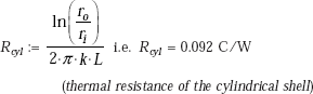
Therefore, ![]()
i.e. Q = 4.368 × 10³ W (heat transfer rate/m length.)
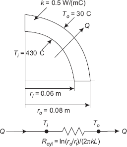
FIGURE Example 4.10 Heat transfer through cylindrical insulation
Temperature at mid-thickness of insulation, i.e. at r = 0.07 m:
Temperature distribution in the cylindrical shell is given by Eq. 4.35,
Temperature profile in the insulation:
In Mathcad, this is very easy to draw. We already have expression for T(r), i.e. temperature as a function of r. Let us define the range variable r, starting from r = 0.06 m to r = 0.08 m, varying in steps of 0.001 m. Then, from the graph palette choose x – y graph, fill in r in the place holder of x-axis and T(r) in the place holder of y-axis. Click anywhere outside the graph region and the graph appears immediately: See Fig. Ex. 4.10(b)
r = 0.06, 0.061, ..., 0.08 |
(define range variable, r; first value = 0.06, next value = 0.061 m, last value = 0.08 m) |
Obviously, temperature distribution is logarithmic, as seen from the expression for T(r).
4.8 Composite Cylinders
Composite cylinders belong to a practically important category, e.g. lagged pipes carrying steam or other high temperature fluids, insulated pipes carrying coolant or cryogenic fluids, insulated tanks, etc. and, these are analysed as composite cylinders.
Consider a system of composite cylinders as shown in Fig. 4.9.
A cylinder of inner radius r1, outer radius r2 and thermal conductivity k1 is covered with another layer (say, insulation) of radius r3 and thermal conductivity k2. There is perfect thermal contact at the interface between the two layers, i.e. there is no temperature drop at the interface. Let T2 be the interface temperature. Further, let a hot fluid at a temperature Ta flow through the inner pipe with a heat transfer coefficient ha. On the outside, let the heat be lost to a cold fluid at a temperature Tb flowing with a heat transfer coefficient of hb. Let L be the length of the cylindrical system.
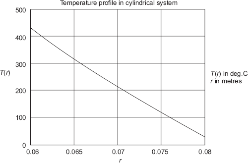
FIGURE Ex. 4.10(b)
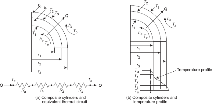
FIGURE 4.9 Composite cylinders, equivalent themal circuit and temperature profile
Assumptions:
- Steady state heat flow
- One-dimensional conduction in the r direction only
- No internal heat generation
- Perfect thermal contact between layers.
Heat transfer occurs from inside to outside in the positive r direction, i.e. heat transfer occurs by convection from the hot fluid at Ta to the inner wall of inner cylindrical layer at T1, then by conduction through the inner cylindrical layer, again by conduction through the outer cylindrical layer and finally by convection from outer wall of outer cylindrical layer at T3 to the cold fluid at Tb.
Under the given stipulations, it is clear that heat flow rate, Q through each layer is the same.
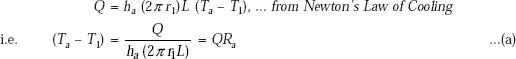
Let us write separately the heat flow equations for these 4 layers:
Convection from the hot fluid to inner wall at T1:
Conduction through first cylindrical layer:
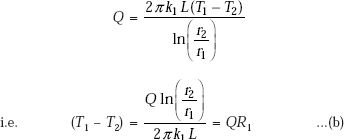
Conduction through second cylindrical layer:
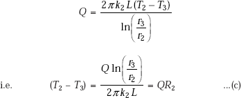
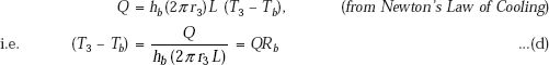
Convection from the outer wall at T3 to cold fluid at Tb:
If there are N concentric cylinders, we can write,
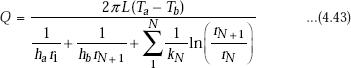
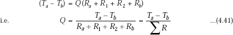
Basically, remember that in the composite cylindrical system just studied, the various resistances such as the two convective resistances and the two conductive resistances are all in series. Then, by analogy with the rules of electrical circuit, total thermal resistance is the sum of the individual resistances. Once these individual resistances are identified and calculated, it is a simple matter to calculate the heat flow rate by analogy with Ohm’s law, i.e. Q = ΔT/Rtotal. Temperatures at the interfaces are calculated by using the fact that Q is the same through each layer and by applying the analogy of Ohm’s law for each layer by turn.
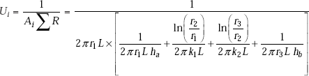
4.9 Overall Heat Transfer Coefficient for the Cylindrical System
Referring to Fig. 4.9, it is clear that heat transfer occurs from hot fluid at Ta to the inner cylinder by convection, then through the inner and outer cylindrical shells by conduction and then to the outer cold fluid at Tb by convection. In many practical applications, the interface temperatures are not known but only the hot and cold fluid temperatures, i.e. Ta and Tb are known. Here, (Ta – Tb) is the overall temperature difference because of which heat flow occurs. We would rather like to write the heat transfer rate in terms of the known overall temperature difference, as follows,
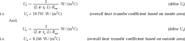
where U is an overall heat transfer coefficient and A is the area normal to the direction of heat flow. In the case of a plane slab, A was a constant with x; however, in the case of a cylindrical system, area normal to the direction of heat flow is 2πrL, and clearly, this varies with r. Therefore, while dealing with cylindrical systems, we have to specify as to which area U is based on, i.e. whether it is based on inside area or outside area. (Generally, U is based on outside area since pipes are specified on outside diameters.)
We write,
where, |
Ui = overall heat transfer coefficient based on inside area |
|
Uo = overall heat transfer coefficient based on outside area |
|
Ai = heat transfer area on inside |
|
Ao = heat transfer area on outside |
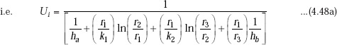
Comparing Eq. 4.44 with Eq. 4.41, we get,
Therefore,
We can also write,
And,
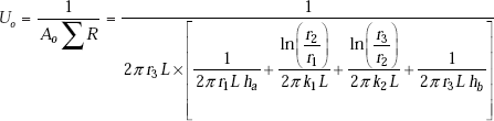
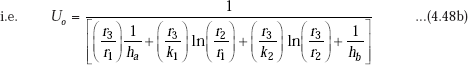
Note: Eqs. 4.48 a and 4.48 b give Ui and Uo in terms of the inside and outside radii. You need not memorise them. To calculate Ui or Uo while solving numerical problems, just remember Eq. 4.46, namely:
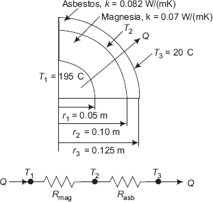
FIGURE Example 4.11 Heat transfer in lagged pipe and the equivalent thermal circuit
Once the total thermal resistance ΣR is calculated, Ui or Uo is easily found out from Eq. 4.46.
The concept of overall heat transfer coefficient in cylindrical systems is often useful in heat exchanger designs, since cylindrical geometry is a popular choice in heat exchangers.
Example 4.11. A 10 cm OD pipe carrying saturated steam at a temperature of 195°C is lagged to 20 cm diameter with magnesia and further lagged with laminated asbestos to 25 cm diameter. The entire pipe is further protected by a layer of canvas. If the temperature under the canvas is 20°C, find the mass of steam condensed in 8 hrs on a 100 m length of pipe. Take thermal conductivity of magnesia as 0.07 W/ (mK) and that of asbestos as 0.082 W/(mK). Neglect the thermal resistance of the pipe material.
(M.U. Dec. 1997)
Solution.
Data:
r1 := 0.05 m r2 := 0.10 m r3 := 0.125 m L := 100 m T1 := 195°C T3 := 20°C kasb := 0.082 W/mK kmag := 0.07 W/mK
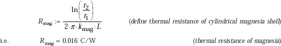
Thermal resistances:
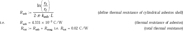
Heat transfer rate, Q:
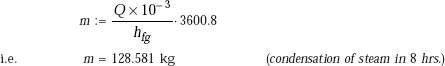
To calculate steam condensed in 8 hrs:
hfg := 1951 kJ/kg |
(latent heat of evaporation for steam at 195°C…from Steam Tables) |
Therefore,
Note: If we need to calculate the interface temperature T2, apply the equivalent Ohm’s law, keeping in mind that heat transfer rate through each layer is constant. For magnesia layer, wer can write: Q = (T1 – T2)/Rmag.
To calculate interface temperature, T2:
From Q = (T1 − T2)/Rmag, we get:
|
T2 := T1 − Q·Rmag, C |
(temperature at the interface) |
i.e. |
T2 = 57.725°C |
(temperature at the interface) |
Check: with reference to the asbestos layer, Q = (T2 – T3)/Rasb. Verify this:
Heat transfer through asbestos layer:
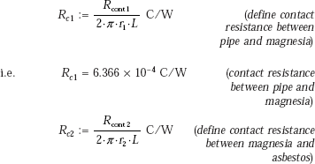
Example 4.12. If in Example 4.11, there is a contact resistance of 0.02 (m2K)/W between the pipe surface and magnesia, and 0.05 (m2K)/W at the interface between magnesia and asbestos, calculate the new value of heat transfer rate. Also, calculate the temperature drops at the two interfaces.
Solution.
Data:
r1 := 0.05 m r2 := 0.10 m r3 := 0.125 m L := 100 m T1 := 195°C T3 := 20°C kasb := 0.082 W/mK kmag := 0.07 W/mK Rcont1 := 0.02 m2K/W (contact resistance between pipe and magnesia)
Rcont2 := 0.05 m2K/W (contact resistance between magnesia and asbestos)
Equivalent thermal circuit and temperature profiles are shown in Fig. Example 4.12.
Thermal resistances:
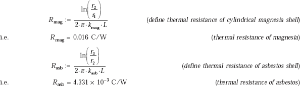
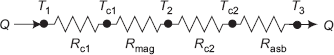
FIGURE Example 4.12(a) Equivalent thermal circuit including contact resistances
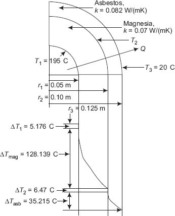
FIGURE Example 4.12(b) Temperature profile in the layers
Contact resistances:
Between the pipe surface and magnesia, contact resistance is given as Rcont1 = 0.02 (m2K)/W; note that this resistance is per m2 of surface. Actual surface area is (2πr1) L. Therefore, contact resistance Rc1 = 0.02/(2πr1L), K/W.
Similarly, at the interface between magnesia and asbestos, contact resistance is given as the 0.05 (m2K)/W and the surface area at the interface is (2πr2L) and therefore, contact resistance Rc2 = 0.05/(2πr2L), K/W.
i.e.
Rc2 = 7.958 × 10⁻⁴ C/W |
(contact resistance between magnesia and asbestos) |
Therefore,
|
Rtotal = Rasb + Rmag + Rc1 + Rc2 C/W |
(total thermal resistance) |
i.e. |
Rtotal = 0.022 C/W |
|
Heat transfer rate, Q:
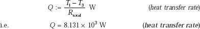
Note that as a result of including the thermal contact resistances, obviously the total resistance to heat flow increases and the new value of heat transfer rate is reduced to 8131 W from the earlier value of 8710 W.
Temperature drops at the interface:
Let ΔT1 be the temperature drop at interface 1, i.e. between pipe surface and magnesia and ΔT2, the temperature drop at interface 2, i.e. between magnesia and asbestos. From analogy with Ohm’s law, we have:
|
ΔT1 := Rc1·Q°C |
(temperature drop at interface between pipe and magnesia) |
i.e. |
ΔT1 = 5.176°C |
(temperature drop at interface between pipe and magnesia) |
And,
|
ΔT2 := Rc2·Q°C |
(temperature drop at interface between magnesia and asbestos) |
i.e. |
ΔT2 = 6.47°C |
(temperature drop at interface between magnesia and asbestos) |
Also,
|
ΔTmag := Rmag·Q°C |
(temperature drop in magnesia layer) |
i.e. |
ΔTmag = 128.139°C |
(temperature drop in magnesia layer) |
|
ΔTasb := Rasb°Q°C |
(temperature drop in asbestos layer) |
i.e. |
ΔTasb = 35.215°C |
(temperature drop in asbestos layer) |
Check: Total temperature drop must be equal to (195 – 20) = 175°C. Verify this:
|
ΔTtotal = ΔT1 + ΔTmag + ΔT2 + ΔTasb |
(define total ΔT |
i.e. |
ΔTtotal = 175°C |
(total temperature drop…verified.) |
Example 4.13. A metal (k = 45 W/(mC)) steam pipe of 5 cm ID and 6.5 cm OD is lagged with 2.75 cm radial thickness of high temperature insulation having thermal conductivity of 1.1 W/(mC). Convective heat transfer coefficients on the inside and outside surfaces are hi = 4650 W/(m2K) and ho = 11.5 W/(m2K), respectively. If the steam temperature is 200°C and the ambient temperature is 25°C, calculate:
- heat loss per metre length of pipe
- temperature at the interfaces, and
- overall heat transfer coefficients referred to inside and outside surfaces (i.e. calculate Ui and Uo).
Solution. This is a case of steady state, one-dimensional heat transfer with no internal heat generation in any of the layers. So, thermal resistance concept is applicable and is used to find out the rate of heat transfer, Q. Also, the principle that Q is the same through each layer is used along with the equivalent Ohm’s law to determine the temperatures at the interfaces. Overall heat transfer coefficients are determined by applying Eq. 4.46, namely,
See Figure Example 4.13.
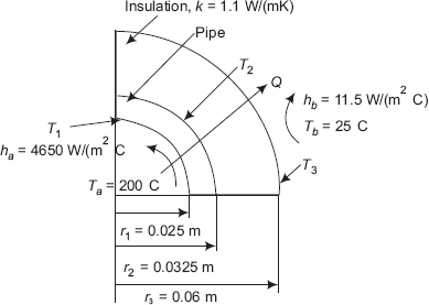
FIGURE Example 4.13(a) Lagged steam pipe, with convection
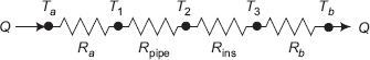
FIGURE Example 4.13(b) Equivalent thermal circuit
Data:
r1 := 0.025 m r2 := 0.0325 m r3 := 0.06 m kpipe := 45 W/(mK) kins := 1.1 W/(mK) L := 1 m Ta := 200°C Tb := 25°C hi := 4650 W/(m2K) ho := 11.5 W/(m2K)
Thermal resistances:
Heat transfer occurs from the inside to outside, as shown in Fig. Example 4.14. Starting from inside, first there is convective resistance between steam and the pipe surface, then conductive resistances through the pipe material and insulation, then again, convective resistance between the outer surface and the ambient. Let us calculate these resistances, by turn:
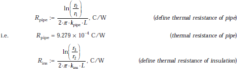
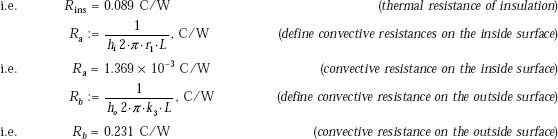
Therefore, total resistance:
|
Rtot := Rpipe + Rins + Ra + Rb, C/W |
(since all resistances are in series) |
i.e. |
Rtot = 0.322 C/W |
(total thermal resistance) |
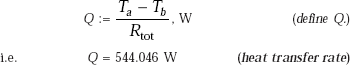
Heat transfer rate, Q is equal to overall temperature difference divided by total thermal resistance, by analogy with Ohm’s law
Temperatures at the interfaces:
For each layer, Q is the same and is equal to the temperature drop through that layer divided by the thermal resistance of that particular layer. Apply this for the inside convective layer, the two conductive layers through pipe and insulation, and then again, the convective layer on the outside, by turn:
(Ta − T1) = Q.Ra
(T1 − T2) = Q.Rpipe
(T2 − T3) = Q.Rins
(T3 − Ta) = Q.Rb
We get:
|
T1 := Ta − Q·Ra°C |
(define T1) |
i.e. |
T1 = 199.255°C |
(temperature of inside surface of pipe) |
|
T2 := T1 − Q·Rpipe°C |
(define T2) |
i.e. |
T2 = 198.75°C |
(temperature of interface of pipe and insulation) |
|
T3 := T2 − Q·Rins°C |
(define T3) |
i.e. |
T3 = 150.489°C |
(temperature of outer surface of insulation) |
Finally, check for value of Tb:
|
Tb := T3 − Q·Rb°C |
(define Tb) |
i.e. |
Tb = 25°C |
(matches with the data…verified) |
Overall heat transfer coefficients, Ui and Uo:
Overall heat transfer coefficients are determined by applying Eq. (4.46), namely, UiAi = UoAo = 1/Σ R: Remember: Ai = 2 πr1.L and Ao = 2 πr3.L
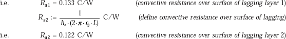
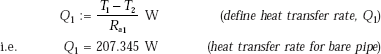
Example 4.14. A 160 mm dia pipe carrying saturated steam is covered by a layer of lagging of thickness 40 mm (k = 0.8 W/(mC)). Later, an extra layer of lagging of 10 mm thickness (k = 0.12 W/(mC)) is added. If the surrounding temperature remains constant and heat transfer coefficient for both lagging materials is 10 W/(m2K), determine the percentage change in rate of heat loss due to the extra lagging layer.
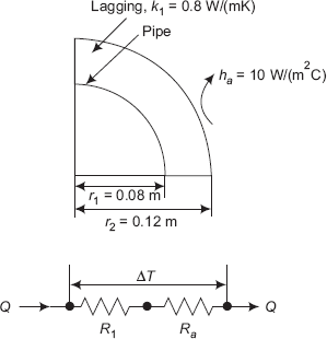
FIGURE Example 4.14(a) Pipe with one layer of lagging
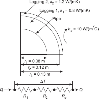
FIGURE Example 4.14(b) Pipe with two layer of lagging
Solution. See Fig. Example. 4.14.
r1 := 0.08 m r2 := 0.12 m r3 := 0.13 m k1 := 0.8 W/(mC) k2 := 0.12 W/(mC) ha:= 10 W/(m2C) L := 1 m
Since this is a case of steady state, one-dimensional conduction with no internal heat generation, thermal resistance concept is applicable.
In case (i): Thermal resistance is the sum of conduction resistance in lagging layer number 1 and convective resistance over its surface. Conduction resistance of the pipe material and the convective resistance between steam and inner surface of pipe are neglected, since no data is given. See Fig. Example. 4.14a.
In case (ii): Thermal resistance is the sum of conduction resistances in lagging layers number 1 and number 2 and the convective resistance over the surface of lagging layer number 2.
Obviously, Rtotal for case (ii) is more than that for case (i); accordingly, heat transfer rate for the second case, Q2 is less than that for first case, Q1.
From analogy with Ohm’s law, we write:
Q1 = ΔT/Rtot1 and Q2 = ΔT/Rtot2 where ΔT is the overall temperature difference, which is the same for both cases.
Therefore, Q1/Q2 = (Rtot1/Rtot2) .
And, % change in heat flow rate = (Q1 – Q2) × 100/Q1 = [1 – (Q2/Q1)] × 100
Thermal resistances:
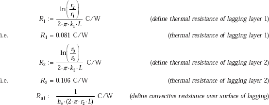
Total resistances:
Case (i): with lagging layer 1 only:
Rtot 1 := R1 + Ra1 i.e. Rtot 1 = 0.213 C/W (total resistance for case (i))
Case (ii): with lagging layer 1 and 2:
Rtot 2 := R1 + R2 + Ra2 i.e. Rtot 2 = 0.309 C/W (total resistance for case (ii))
Percentage change in heat transfer rate:
First, find out (Q2/Q1 from: (Q2/Q1 = (Rtot1/Rtot2)
And,
|
Per cent change := (1 − Q2 by Q1)·100 |
(define % change) |
i.e. |
Per cent change = 31.029 |
i.e. change in heat transfer rate is 31.029%. |
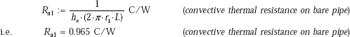
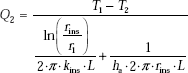
Example 4.15. A 3.3 cm OD steel pipe, outside surface of which is at 500 K, is surrounded by still air at 300 K. The heat transfer coefficient by natural convection is 10 W/(m2K). It is proposed to reduce the heat loss to half by applying magnesia insulation (k = 0.07 W/(mK) on the outside surface of the pipe. Determine the thickness of the insulation. Assume pipe surface temperature and convective heat transfer coefficients remain the same.
Solution. Thermal resistance concept is applicable since it is a case of steady state, one-dimensional conduction, with no internal heat generation.
There are two cases:
Case (i): Without insulation, i.e. bare pipe-now, the heat transfer occurs only by natural convection on the pipe surface and the heat transfer rate, Q1 is given by Newton’s Law of Cooling, namely, Q1 = ha (2πr1. L).ΔT, or, Q1 = ΔT/Ra1, where Ra1 is the convective resistance and ΔT = (500 – 300) deg.
Case (ii): With insulation: Now, the heat transfer rate, Q2 is given to be half of Q1. Thermal resistances involved are: the conductive resistance of the cylindrical insulation layer (= R1) and the convective resistance over the insulation surface (= Ra 2).
i.e. Q2 = ΔT/(R1 + Ra2). Write the expression for Q2 and solve the resulting transcendental equation by trial and error to get the outer radius of insulation.
Situations of case (i) and (ii) are depicted in Fig. Example. 4.15(a) and (b).
Data:
r1 := 0.0165 m ha := 10 W/(m2K) kins := 0.07 W/(mC) T1 := 500 K T2 := 300 K L := 1 m
Let rins be the outer radius of insulation
Case (i): bare pipe:
Therefore,
Case (ii): pipe with insulation:
Now,
We have: |
Q2 = ΔT/ΣR, |
i.e. |
Q2 = ΔT/(R1 + Ra2) |
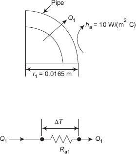
FIGURE Example 4.15(a) Pipe without insulation
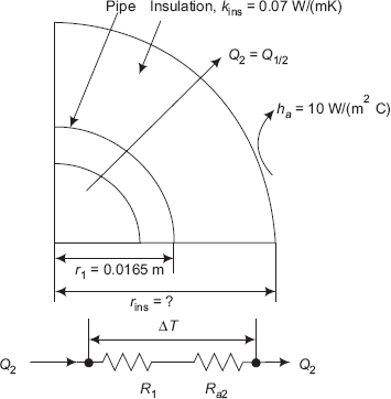
FIGURE Example 4.15(b) Pipe with insulation
So, we get:
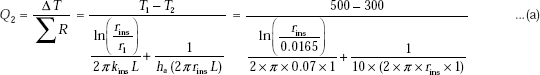
Simplifying, we get:
This equation has to be solved to get rins; and, trial and error solution is required since it is a transcendental equation. Solve it by hand, as an exercise.
However, it is easily solved in Mathcad, using solve block. Start with a trial value of rins and write the constraint (i.e. Eq. (a)) immediately below ‘Given’; then the command Find(rins) gives the value of rins: Note that you need not even simplify Eq. (a).
Given
|
Find(rins) = 0.030683 |
|
i.e. |
rins := 0.0307 m |
(outer radius of insulation) |
Therefore, thickness of insulation:
|
tins := rins − r1 m |
(define thickness of insulation) |
i.e. |
tins = 0.014 m |
(thickness of insulation) |
4.10 Spherical Systems
Spherical system is one of the most commonly used geometries in industry. It finds its applications as storage tanks, reactors, etc. in petrochemical, refineries and cryogenic industries. Sphere has minimum surface area for a given volume and material requirement to manufacture a sphere is minimum compared to other geometries.
Here, let us analyse the spherical shell for heat transfer in one-dimensional conduction, i.e. it is assumed that temperature gradients are significant only in the radial direction; so, heat flow occurs only in the radial direction. Now, here also, as in the case of a cylindrical system, the area normal to the direction of heat flow is not a constant, but varies with r.
Consider a spherical shell, inside radius ri and outside radius ro. Inner and outer surfaces are at uniform temperatures of Ti and To, respectively. See Fig. 4.10.
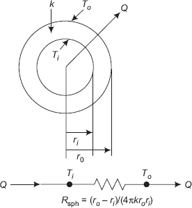
FIGURE 4.10(a) Spherical system and the equivalent thermal circuit
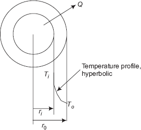
FIGURE 4.10(b) Variation of temperature along the radius
Assumptions:
- Steady state conduction
- One-dimensional conduction, in the r direction only
- Homogeneous, isotropic material with constant k
- No internal heat generation.
Now, since we are considering a spherical system, it is logical that we adopt spherical coordinates. General differential equation for conduction in spherical coordinates is given by Eq. 3.21. For the above mentioned assumptions, Eq. 3.21 reduces to:
Note that now, it is not partial derivative, since there is only one variable, r.
We have to solve this differential equation to get the temperature distribution along r and then apply Fourier’s law to calculate the heat flux at any position.
Multiplying Eq. 4.49 by r2,
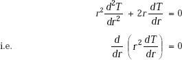
Integrating,
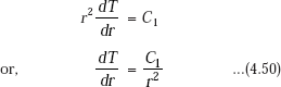
Integrating again,
where, C1 and C2 are constants of integration.
Eq. 4.51 gives the temperature distribution in the spherical shell as a function of radius.
C1 and C2 are found out by applying the two B.C.’s:
- at r = ri, T = Ti
- at r = ro, T = To
B.C. (i) gives: |
Ti = − C1/ri + C2 |
…(a) |
B.C. (ii) gives: |
To = − C1/ro + C2 |
…(b) |
and, from Eq. a:
Substituting C1 and C2 in Eq. 4.51, we get
Eq. 4.52 is the desired equation for temperature distribution along the radius.
Eq. 4.52 is written in non-dimensional form as follows:
Temperature distribution for the spherical system is shown in Fig. 4.10 (b). Note that the temperature distribution is a hyperbola.
Next, to find the heat transfer rate, Q:
We apply the Fourier’s law. Since it is steady state conduction, with no heat generation, Q is the same through each layer.
Considering the outer surface, i.e. at r = ro
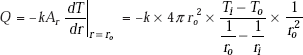
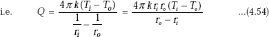
Eq. 4.54 gives the desired expression for rate of heat transfer through the spherical system. Now, writing Eq. 4.54 in a form analogous to Ohm’s law:
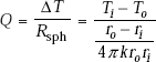
Immediately, we observe that thermal resistance for conduction for a spherical shell is given by:
Alternatively
Since it is steady state, one-dimensional conduction, with no heat generation, heat flow rate, Q is constant at every cross-section; so, we can directly integrate Fourier’s equation between the two known temperatures (and the corresponding, known radii), keeping Q out of the integral sign; this will give us Q. Then, at any r, the temperature T(r) is calculated by integrating between r = ri and r = r (with T = Ti and T = T(r)), and equating the Q obtained now to the expression for Q obtained earlier.
Refer to Fig. 4.11.
At any radius r, consider an elemental spherical shell of thickness dr; let the temperature differential across this thin layer be dT. Then, in steady state, rate of heat transfer through this layer Q, can be written from Fourier’s law, to be equal to:
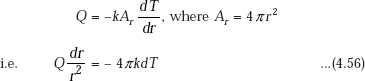
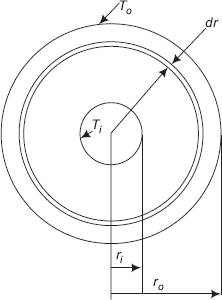
FIGURE 4.11 Spherical system
Integrating Eq. 4.56 from ri to ro (with temperature from Ti to To),
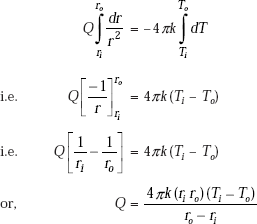
…same as Eq. 4.54
To get the temperature profile within the spherical shell:
At any radius r, let the temperature be T(r).
s
Integrating Eq. 4.56 from ri to r, i.e. replace ro by r and To by T(r) in Eq. 4.54,
Now, apply the principle that Q is the same through each layer, i.e. equate Eqs. 4.54 and 4.57:
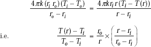
(same as Eq. 4.53)
Concept of “geometric mean area” for a spherical system:
As in the case of the cylindrical system, it is convenient to think of an equivalent slab for the spherical system, i.e. we would like to express the thermal resistance of the sphere in the form of the thermal resistance for a slab (i.e. R = L/(kA)). If we define L as the thickness of the spherical shell, i.e. Lsph = (ro – ri), we can write from Eq. 4.55:
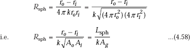
i.e. thermal resistance of spherical shell, Rsph is expressed in a form analogous to that of a plane slab. Here, the equivalent area, ![]() , are the outer and inner surface areas, respectively, of the spherical shell.
, are the outer and inner surface areas, respectively, of the spherical shell.
Note: It is very common that containers have hemispherical ends. Then, remember that thermal resistance of a hemispherical spherical shell is half that of a spherical shell as given by Eq. 4.55.
Example 4.16. Consider an aluminium hollow sphere of inside radius ri = 2 cm, outside radius ro = 6 cm and k = 200 W/ (mC). The inside surface is kept at an uniform temperature of Ti = 100°C and outside surface dissipates heat by convection with h = 80 W/(m2C) into ambient air at a temperature of Ta = 20°C. Determine:
- outside surface temperature of the sphere in steady state
- rate of heat transfer
- temperature within the aluminium sphere at a radius r = 3 cm
- sketch the temperature distribution along the radius.
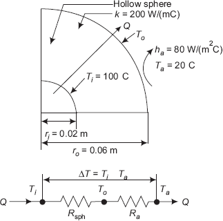
FIGURE Example 4.16 Hollow sphere with convection
Solution. See Fig. Example. 4.16.
Data:
ri := 0.02 m ro := 0.06 m k := 200 W/(mC) Ti := 100°C Ta := 20°C h := 80 W/(m2C)
Let To be the temperature of outside surface of spherical shell.
Since it is a case of steady state, one-dimensional heat transfer with no internal heat generation, thermal resistance concept is applicable.
Heat transfer through the sphere is by conduction and then, from the outer surface of the sphere to ambient, it is by convection. So, calculate these resistances, i.e. Rsph is given by Eq. 4.55 and convective resistance, Ra = 1/(h.Ao), where Ao = (4πro2) is the outer surface area of the spherical shell. Now, apply the equivalent Ohm’s law, i.e. Q = ΔT/Rtot to get the heat transfer rate, Q. See Fig. Example 4.16 for equivalent thermal circuit.
Thermal resistances:
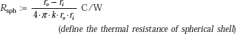
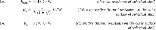
Total thermal resistances:
Therefore, |
Rtot := Rsph + Ra C/W |
(define total thermal resistance) |
i.e. |
Rtot = 0.29 C/W |
(total thermal resistance) |
Heat thermal rate, Q
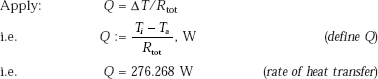
Temperature of outer surface of spherical shell:
Apply the equivalent Ohm’s law only to the convective layer, remembering that Q is same through each layer in steady state, i.e. Q = (To – Ta)/Ra. Therefore,
To = Ta + Q.Ra
We have: To := Ta + Q.Ra, (define To)
i.e.
To = 96.336 C (temperature of outer surface of shell)
Verify with reference to the spherical shell:
we get:
Temperature at a radius of r = 3 cm:
Temperature distribution along the radius is given by Eq. 4.53, namely,
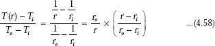
Therefore, we get:
Now, substitute r = 0.03 in T (r) to get temperature at that radius:
i.e. T(0.03) = 98.168°C (temperature at a radius of 0.03 m)
Temperature profile along the radius:
This is drawn very easily in Mathcad. First, define a range variable r varying from inner radius to outer radius, i.e. from 0.02 m to 0.06 m, say at an interval of 0.001 m. Then, choose the x – y graph from the graph palette. Fill in the place holders on the x-axis and y-axis with r and T (r), respectively. Click anywhere outside the graph region and ilmmediately the graph appears: See Fig. Ex. 4.16(b)
r := 0.02, 0.021, …, 0.06 |
…define range variable r; starting value of r = 0.02, next value = 0.021 and last value of r = 0.06 m |
Note: verify from the graph that temperature at r = 3 cm is, indeed, 98.168 deg.C.
4.11 Composite Spheres
Assumptions:
- Steady state heat flow
- One-dimensional conduction in the r direction only
- No internal heat generation
- Perfect thermal contact between layers.
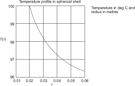
FIGURE Ex. 4.16(b)
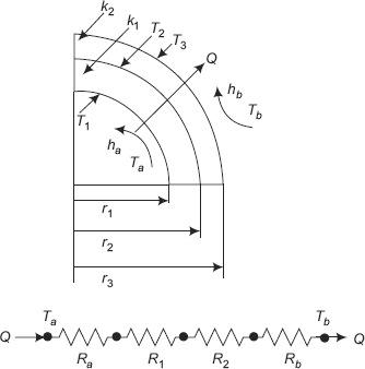
FIGURE 4.12(a) Composite spheres and equivalent thermal circuit
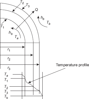
FIGURE 4.12(b) Composite spheres and temperature profile
Consider a system of composite cylinders as shown in Fig. 4.12.
A hollow sphere of inner radius r1, outer radius r2 and thermal conductivity k1 is covered with another layer (say, insulation) of radius R3 and thermal conductivity k2. There is perfect thermal contact at the interface between the two layers, i.e. there is no temperature drop at the interface. Let T2 be the interface temperature. Further, let a hot fluid at a temperature Ta transfer heat to the inner sphere with a heat transfer coefficient ha. On the outside, let the heat be lost from the surface at a temperature of T3 to a cold fluid at a temperature Tb flowing with a heat transfer coefficient of hb.
Under the given stipulations, it is clear that heat flow rate, Q through each layer is the same. Let us write separately the heat flow equations for the 4 layers:
Convection from the hot fluid to inner wall at T1:
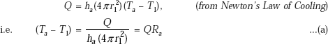
Conduction through first spherical layer:
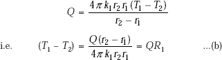
Conduction through second spherical layer:
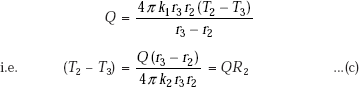
Convection from the outer wall at T3 to cold fluid at Tb:
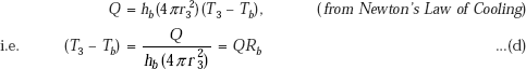
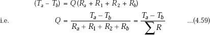
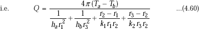
If there are N concentric spheres, we can write:
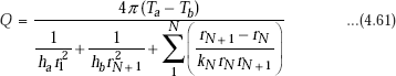
Basically, remember that in the composite spherical system just studied, the various resistances such as the two convective resistances and the two conductive resistances are all in series. Then, by analogy with the rules of electrical circuit, total thermal resistance is the sum of the individual resistances. Once these individual resistances are identified and calculated, it is a simple matter to calculate the heat flow rate by analogy with Ohm’s law, i.e. Q = ΔT/Rtotal. Temperatures at the interfaces are calculated by using the fact that Q is the same through each layer and by applying the analogy of Ohm’s law for each layer by turn.
4.12 Overall Heat Transfer Coefficient for the Spherical System
As in the case of cylindrical systems, we define an overall heat transfer coefficient for the spherical systems also. Again, in this case too, the area normal to the direction of heat flow varies with the radius and it is necessary to specify as to on which area the overall heat transfer coefficient is based.
Accordingly, we write:
where, |
Ui |
= overall heat transfer coefficient based on inside area |
|
Uo |
= overall heat transfer coefficient based on outside area |
|
Ai |
= heat transfer area on inside |
|
Ao |
= heat transfer area on outside |
Therefore, we get:
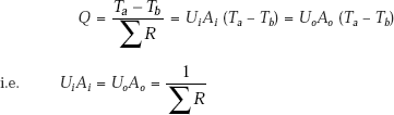
Therefore,
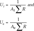
We can also write:
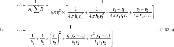
And,
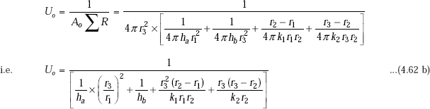
Note: Eqs. 4.62 a and 4.62 b give Ui and Uo in terms of the inside and outside radii. You need not memorise them. To calculate Ui or Uo while solving numerical problems, just remember Eq. 4.46, namely
Example 4.17. A spherical vessel containing hot fluid at 160°C is of 0.4 m OD and is made of titanium of 25 mm thickness. The thermal conductivity is 20 W/(mK). The vessel is insulated with two layers of 5 cm thick insulations of thermal conductivities 0.06 and 0.12 W/(mK). There is a contact resistance of 6 × 10⁻⁴ and 5 × 10⁻⁴ (m2C)/W between the metal and first insulation and between the insulating layers. The outside is exposed to surrounding at 30°C with a convection coefficient of 15 W/(m2K). Determine the rate of heat loss, the interface temperatures and the overall heat transfer coefficients based on inside surface area as well as outside surface area (i.e. calculate Ui and Uo).
Solution. See Fig. Ex. 4.17(a) & (b).
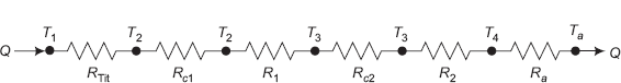
FIGURE Example 4.17(a) Equivalent thermal circuit including contact resistances
Data:
r1 := 0.175 m r2 := 0.20 m r3 := 0.25 m r4 := 0.30 m kTit := 20 W/(mK) k1 := 0.06 W/(mK) k2 := 0.12 W/(mK) T1 := 160°C Ta := 30°C ha := 15 W/(m2K) Rcont1 := 6 × 10⁻⁴ m2C/W Rcont2 := 5 × 10⁻⁴ m2C/W
Thermal resistances:
Thermal resistance network is shown in Fig. Example 4.17(a).
Conductive resistances:
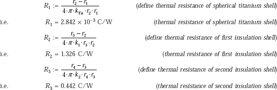
Convective resistances:

Contact resistances:
Between the titanium surface and first insulation, contact resistance is given as Rcont1 = 6 × 10⁻⁴ (m2C)/W; note that this resistance is per m2 of surface. Actual surface area is (4 πr22). Therefore, contact resistance Rc1 = 6 × 10⁻⁴/(4πr22), C/W
Similarly, at the interface between the two insulation layers, contact resistance is given as 5 × 10⁻⁴ (m2C)/W and the surface area at the interface is (4 πr32) and therefore, contact resistance Rc2 = 5 × 10⁻⁴/(4 πr32), C/W
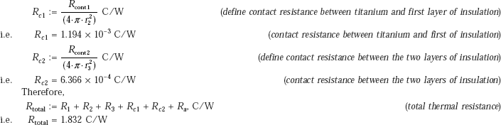
Heat transfer rate, Q:
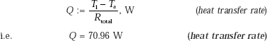
Interface temperatures:
To calculate the interface temperatures, let us calculate the temperature drop through each layer, starting from the inner titanium layer, i.e. ΔT = Q.R, from Ohm’s law. Also, remember that Q is the same through each layer.
Temperature drops at the interfaces:
Let Δ TTit be the temperature drop in the titanium metal layer and Δ Tc1, the temperature drop at the interface 1 between titanium and first insulation layer, and Δ T1, the temperature drop through the first insulation layer, and Δ Tc2, the temperarture drop at the interface 2 between the two insulation layers, and Δ T2 the temperature drop through the second insulation layer, and Δ T3, the temperature drop in the outer convection layer.
From analogy with Ohm’s law, we have:
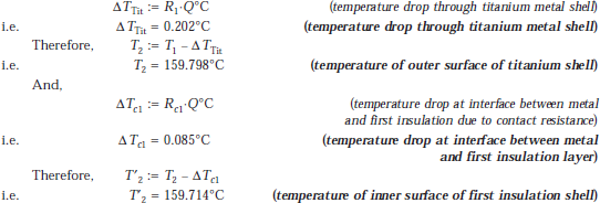
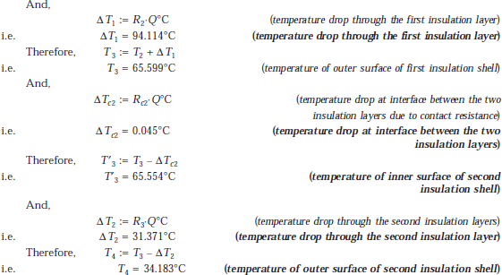
Check: Considering the outer convective layer, and applying Ohm’s law, we should get Q = (T4 – Ta)/Ra. This should equal 70.96 W, obtained earlier. Verify this:
Temperature profile is shown in Fig. Example 4.17(b):
Overall heat transfer coefficients, Ui and Uo:
Remember that: UiAi = U0.A0 = 1/Σ R
where, Ai and Ao are the inner and outer surface areas of spherical shells, respectively.
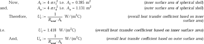
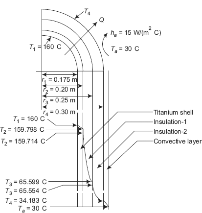
FIGURE Example 4.17(b) Temperature profile in the layers
i.e. Uo = 0.483 W/(m2C) (overall heat transfer coefficient based on outer surface area)
Note: We can also write: Uo = Ui × (Ai/Ao).
4.13 Critical Thickness of Insulation
Insulation is added to a surface to reduce the heat loss from the surface to the ambient, if the surface is hot, or to reduce the heat loss into the surface from the ambient, if the surface is cold. Either way, the aim is to reduce the heat loss. Generally, addition of insulation does reduce the heat loss; however, there are some interesting cases where this may not be so, and the addition of insulation, in fact, increases the heat loss!
To get an insight into such a possibility, let us consider following two cases:
Case (i): Insulating a cubical furnace. Let the furnace wall be at a high temperature of T1. Insulation is provided over this wall to reduce the heat loss to the ambient, which is at a temperature of Ta. Furnace wall loses heat to the surroundings by conduction through the insulation layer and by convection from the outer surface of insulation. So, the resistance to heat transfer is made up of two components, namely, conductive resistance of the insulation slab (= L/(kA)) and convective resistance between the wall surface and the surroundings (= 1/(h.A)), where L is the thickness of the insulation slab, k its thermal conductivity and h is the heat transfer coefficient for convection. A is the area normal to the direction of heat flow, which is a constant for a slab configuration. Obviously, as the insulation thickness is increased, its conductive resistance increases and the convective resistance remains constant and therefore, the total resistance increases; as a result, the heat loss goes on decreasing as the insulation thickness goes on increasing.
Case (ii): Insulating a pipe carrying a hot fluid. Let the pipe wall be at a high temperature of T1. Insulation is provided over this wall to reduce the heat loss to the ambient, which is at a temperature of Ta. Pipe wall loses heat to the surroundings by conduction through the insulation layer and by convection from the outer surface of insulation. So, the resistance to heat transfer is made up of two components, namely, conductive resistance through the cylindrical insulation layer [= ln(r2/r1)/(2 π kL)] and convective resistance between the wall surface and the surroundings [= 1/(h.Ao)], where r1 is the inner radius of insulation layer (or, outer radius of pipe), r2 is the outer radius of insulation layer, k its thermal conductivity, L is length of pipe, and h is the heat transfer coefficient for convection. Ao is the area of outer surface of insulation. Obviously, as the insulation thickness is increased, i.e. as insulation radius r2 is increased, conductive resistance of insulation increases; however, convective resistance, given by [1/(h. Ao)] goes on decreasing since Ao, the outside surface area goes on increasing with increasing radius. Therefore, the total resistance may increase or decrease, depending on the relative rates of change of these two resistances. And, there are situations where the total resistance does decrease as the insulation thickness increases i.e. the heat transfer rate Q increases as the thickness is increased! Let us analyse when this happens.
For the above case, the equivalent thermal resistance circuit is shown below in Fig. 4.13 (a). Consider any radius r of the insulation. Let us investigate the variation of the two resistances and therefore, of Q, as the insulation radius r varies:
The total temperature potential for heat flow is (T1 – Ta). The resistances involved are:
- Rins = conductive resistance of the cylindrical insulation layer
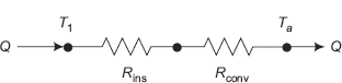
FIGURE 4.13(a) Equivalent thermal circuit for a cylinder with insulation
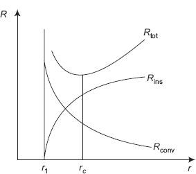
FIGURE 4.13(b) Variation of resistances with insulation radius for a cylinder
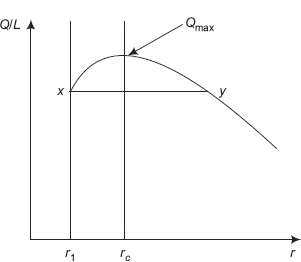
FIGURE 4.13(c) Heat transfer per unit length vs. insulation radius for a cylinder
i.e.
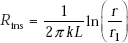
and,
- Rconv = convective resistance on the surface of insulation, i.e. at radius r.
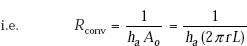
As stated earlier, conduction resistance, Rins increases as r increases, and, convection resistance, Rconv decreases as r increases. Variation of Rins and Rconv with r are shown in Fig. 4.13(b); this figure also shows the variation of the total resistance, Rtot given by:
Note that Rtot passes through a minimum. The insulation radius at which the resistance to heat flow is minimum is called ‘critical radius’, rc; i.e. the heat flow is a maximum at the critical radius.
Correspondingly, the variation of heat flow per unit length, (Q/L), with r is shown in Fig. 4.13(c):
In Fig. 4.13 (c), r1 is the radius of the bare pipe and the value of Q/L at this point is the heat transfer rate per unit length for the bare pipe. Insulation is added over the pipe and till the insulation radius r reaches the value of rc, Q/L goes on increasing and reaches a maximum at r = rc. As the insulation radius is increased further, Q/L decreases, but is still at value higher than that for the bare pipe. As can be seen from the figure, at point y, value of Q/L is the same as at point x, i.e. the value of Q/L for the bare pipe. Beyond the value of r corresponding to point y, value of Q/L decreases with r and the insulation becomes really effective. It should be noted that when the radius of the pipe r1 is less than that of critical radius rc, the insulation is not really effective in the radius range of r1 to rc, since adding the insulation actually increases the heat flow rate.
Mathematically, to find out at what insulation radius r the Rtot becomes a minimum for the cylindrical system, let us differentiate the expression for Rtot and equate to zero; then, to confirm that at that rc, the Rtot indeed goes through a minimum, verify that the second derivative of Rtot w.r.t. r is positive:
Now,
In the above expression for Rtot, r the external radius of insulation, is the only variable. So, to find out at what value of r the Rtot is minimum, differentiate Rtot w.r.t r and equate to zero:
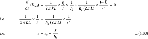
Eq. 4.63 gives the expression for critical radius, rc for the cylindrical system.
To confirm that at r = rc, Rtot indeed is minimum, let us find out the value of (d2Rtot/dr2) at r = rc:
Substituting r = rc = k/ha in the above expression:
It is clear from Eq. 4.64 that (d2Rtot/dr2) at r = rc is +ve i.e. at r = rc, the Rtot is a minimum. There are two cases of practical interest, as shown in Fig. 4.14:
Case (i): rl < rc: This situation is shown in Fig. 4.14 (a).
Here, r1, the radius of the pipe happens to be less than the critical radius. Therefore, addition of insulation increases the heat flow rate (Q/L) till the insulation radius reaches a value of rc, the critical radius (i.e. range a – b in the figure) and beyond this point, further addition of insulation decreases the value of (Q/L). In practice, such a case is likely to occur if insulation material of poor quality is applied to pipes or wires of small radius. This situation is profitably utilised in insulating current carrying wires, where the electrical insulation provided is a material of poor thermal conductivity; here, the radius of the current carrying wire is small and is generally less than the value of critical radius. Thus, addition of electrical insulation actually helps to dissipate more heat from the wire and results in cooling it.
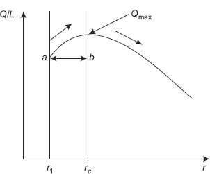
FIGURE 4.14(a) Heat transfer per unit length vs. insulation radius for a cylinder when r1 < rc
Case (ii): r1 > rc: This situation is shown in Fig. 4.14(b).
Here, r1, the radius of the pipe happens to be more than the critical radius. Therefore, addition of insulation decreases the heat flow rate (Q/L) as shown in range (a – b) in the figure. In practice, such a case is applicable in insulation of steam pipes and refrigerant lines. However, it may not be necessary to check for critical radius while insulating steam lines due to the following reason: generally, the value of k for insulations used in those applications is of the order of 0.05 W/(mC), and ha for natural convection is of the order of 5 W/(m2C) and thus the critical radius is of the order of rc = (0.05/5) = 0.01 m, i.e. 1 cm. Often, the pipe radius is more than this value, and addition of insulation will decrease the rate of heat transfer as desired.
Critical thickness of insulation for a sphere. Case of a sphere is similar to that of cylinder since here also, as the radius of insulation increases, the surface area increases. So, as the insulation radius is increased, the conduction resistance of insulation increases and the convection resistance decreases.
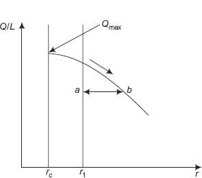
FIGURE 4.14(b) Heat transfer per unit length vs. insulation radius for a cylinder when r1 > rc
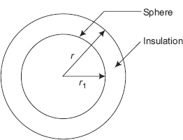
FIGURE 4.15 Critical radius for a sphere
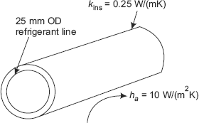
FIGURE Example 4.18 Critical radius for a cylinder
Let r1 be the radius of the sphere on which insulation is applied, and let r be the outer radius of insulation. See Fig. 4.15. We would like to investigate the change of Rtot as insulation radius r is varied:
We have, for the spherical system:
Differentiating Rtot w.r.t. r and equating to zero:
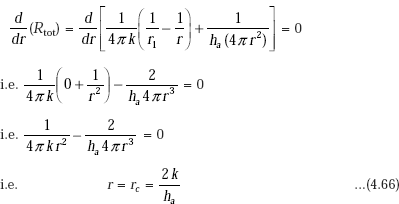
Eq. 4.66 gives the expression for critical radius, rc for the spherical system. (To confirm that at r = rc, Rtot indeed is minimum, check that the value of (d2 Rtot/dr2) at r = rc. is positive. This is left as an exercise to the student.) Therefore, critical thickness of insulation for spherical system = (rc – r1).
Example 4.18. A refrigerant suction line of 25 mm OD is to be insulated using a material of thermal conductivity k = 0.25 W/ (mK). The surface heat transfer coefficient ha is 10 W/(m2K). Verify if the insulation is effective or not. What should be the maximum value of thermal conductivity of insulation to reduce the heat transfer? (M.U. 2000)
Solution.
Data:
r1 := 0.0125 m kins := 0.25 W/(mK) ha := 10 W/(m2K)
Therefore,
Critical radius, rc:
(define critical radius for cylindrical system, from Eq. 4.64)
i.e. rc = 0.025 m (…critical radius)
This value of rc is more than r1, i.e. starting from the refrigerant line surface at radius r1, as we go on increasing the thickness of insulation, Q goes on increasing (instead of decreasing) till we reach a radius of rc.
Therefore, insulation is not effective.
Max value of k to reduce heat transfer:
As the insulation radius exceeds the value of rc, Q starts decreasing. So, the maximum value of the thermal conductivity required for rc to be equal to r1 is given by: kmax = r1 × ha (from rc = k/ha)
i.e. |
kmax := r1×ha |
|
i.e. |
kmax = 0.125 m |
(maximum value of thermal conductivity of insulation to reduce heat transfer) |
Example 4.19. In Example 4.18, calculate the heat loss per metre length for every 2.5 mm increase in thickness of insulation, up to a radius of 34.5 mm. Draw the graph of (Q/L) vs. radius of insulation. Given: temperature of refrigerant line surface, T1 = –20°C and ambient temperature, Ta = 25°C.
Solution.
Data:
r1 := 0.0125 m kins := 0.25 W/(mK) ha := 10 W/(m2K) T1 := 20°C Ta := 25°C L := 1 m
Heat transfer per unit length, Q/L:
Overall temperature difference is ΔT = (T1 – Ta). This value will be negative since T1 is less than Ta, and the heat flow is from outside ambient to inside line surface. So, we write ΔT as (Ta – T1) to make Q positive. The total resistance, Rtot = Rcond + Rconv, where Rcond is the conductive resistance of cylindrical layer of insulation and Rconv is the convective resistance between the insulation surface and the ambient.
We have from Eq. (4.62):
And, for L = 1 m, Q = ΔT/Rtot
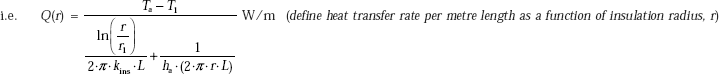
Calculate Q for various values of r:
Let r vary from 12.5 mm to 34.5 m at an increment of 2 mm.
So, define a range variable r to vary through this range. Then, in Mathcad, just give the command ‘r = ’ and a Table of r values appears; also type the command ‘Q(r) = ’ and a Table of Q values at the defined values of r appears. Arrange them side by side:
r = 0.0125, 0.0145, …, 0.0345 |
…define the range variable r; first value = 0.0125 m, next value = 0.0145 m and last value = 0.345 m |
| r | Q(r) |
|---|---|
0.0125 |
35.343 |
0.0145 |
37.748 |
0.0165 |
39.428 |
0.0185 |
40.545 |
0.0205 |
41.235 |
0.0225 |
41.607 |
0.0245 |
41.743 |
0.0265 |
41.707 |
0.0285 |
41.546 |
0.0305 |
41.296 |
0.0325 |
40.983 |
0.0345 |
40.627 |
Above Table gives the values of r and corresponding values of Q(r), side by side.
Observe that starting from the bare refrigerant line, (Q/L) goes on increasing as insulation is applied, reaches a peak at r = 25 mm (i.e. the critical thickness) and then goes on decreasing. It is interesting to note that even with 34.5 mm thickness of insulation, heat transfer per metre is larger than that with no insulation!
Graph of Q(r) vs. r:
This is drawn easily in Mathcad. Range variable, r and heat flow rate per unit length, Q(r) are already defnied. Now, from the Graph palette, choose x – y graph, fill in the place holder on the x-axis with r and that on the y-axis with Q(r) and click outside the graph region. Immediately the graph appears: See Fig. Ex. 4.19
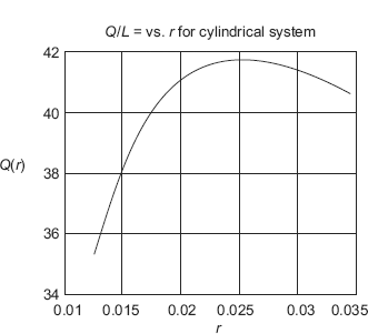
FIGURE Example 4.19
Note that Q(r) passes through a maximum at r = 0.025 m, i.e. at the value of critical radius. Observe the similarity with Fig. 4.13(c).
Example 4.20. A 25 mm OD pipe line is to be thermally insulated with a material of k = 0.25 W/(mK). Heat transfer coefficient for surroundings, ha = 12 W/(m2K). Check whether the insulation would be effective or not. What should be the maximum value of k for the insulating material to effectively reduce the heat transfer? Also, find the thickness of insulation if an alternative material with k = 0.04 W/(mK) is employed and it is desired to reduce the heat transfer to 20.7% of that of bare pipe.
Solution.
Data:
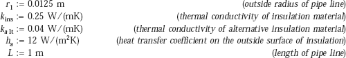
Critical radius, rc:
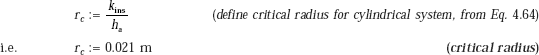
This value of rc is more than r1, i.e. starting from the pipe surface at radius r1, as we go on increasing the thickness of insulation, Q goes on increasing (instead of decreasing) till we reach a radius of rc. Therefore, insulation is not effective.
Max value of k to reduce heat transfer:
As the insulation radius exceeds the value of rc, Q starts decreasing. So, the maximum value of the thermal conductivity required for rc to be equal to r1 is given by: kmax = r1 × ha. (from rc = k/ha)
i.e. |
kmax := r1ha |
|
i.e. |
kmax := 0.15 m |
(maximum value of thermal conductivity of insulation to reduce heat transfer.) |
Thickness of alternative insulation when its k = 0.04 W/(mK):
It is also stated that with this alternative insulation heat transfer rate must be 20.7% of that of the bare pipe. Now, note that for the bare pipe, there is heat transfer only by convection at its surface. Let the convective resistance to heat transfer on the bare surface be Rbare. For the insulated pipe, let the total resistance be Rtot. Obviously, Rtot is made up of conductive resistance of the cylindrical insulation material (Rins) and the convective resistance over its surface (Rconv).,
i.e. Rtot = Rcond + Rconv.
Since the heat transfer with insulation is 20.7% of that for the bare pipe, for the same ΔT, we write:
i.e. |
ΔT/Rtot = 0.207 × ΔT/Rbare |
i.e. |
Rtot = Rbare/0.207 |
Now, |
Rba re = 1/{(2πr1L).ha} |
|
Rcond = ln(ra lt/r1)/(2πka ltL), where ra lt is the radius of alternative insulation |
|
Rconv = 1/(2πra lt ha) |
Thermal resistances:
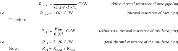
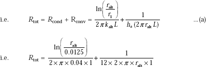
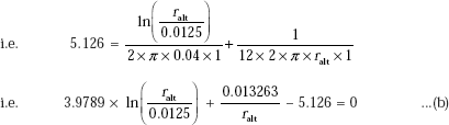
Eq. b is a transcendental equation and has to be solved by trial and error. This is done easily in Mathcad, using solve block. Start with a trial value of ralt then type ‘Given’; and immediately below ‘Given’ type the constraint viz. Eq. b. Then, the command ‘Find (ralt)’ gives the value of ralt. as shown below:
Given
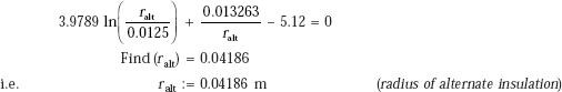
i.e. we get: ra lt, the radius of the alternate insulation = 0.04186 m i.e. 41.86 mm.
Thickness of alternate insulation:
Therefore, thickness of alternate insulation, t, is given by:
|
t := ralt − r1 m |
(define thickness of alternate insulation) |
i.e. |
t = 0.02936 m |
(thickness of alternate insulation.) |
Note: While solving Eq. a, it was first simplified to Eq. b and then Solve block was used. This was done just for clarity. However, while using Mathcad, Eq. a can directly be solved in the Solve block as shown below: (Also see Example 4.15)
Given
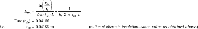
Note: In this case, we took a different trial value of ralt to start with, just to show that it makes no difference in the final value of ralt.
Example 4.21. A wire of 8 mm diameter at a temperature of 60°C is to be insulated by a material having k = 0.174 W/ (mC). Heat transfer coefficient on the outside, ha = 8 W/(m2K). Ambient temperature, Ta = 25°C. For maximum heat loss, what is the minimum thickness of insulation and the heat loss per metre length? Find the increase in heat dissipation due to insulation. Also, calculate the increase in current carrying capacity due to insulation.
(M.U. 2000)
Solution. If r1, the radius of the wire is less than the critical radius rc, then, as the insulation is added on the bare wire, heat loss goes on increasing, and becomes a maximum at the critical radius. So, the problem is to determine the critical radius.
Data:
r1 := 0.004 m kins := 0.174 W/(mC) ha := 8 W/(m2K) T1 := 60°C Ta := 25°C L := 1 m
Critical radius:
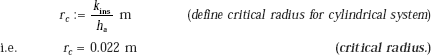
Thickness of insulation for maximum heat transfer:
Maximum heat transfer occurs at the critical radius. Therefore, thickness of insulation at the critical radius is:
|
tins := rc − r1 m |
(define tins) |
i.e. |
tins = 0.01775 m.. = 17.75 mm |
(thickness of insulation) |
Increase in heat transfer rate due to insulation:
Calculate heat loss for the bare wire and insulated wire separately and compare them. Remember: heat loss = ΔT/R Heat loss/m without insulation:
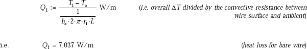
Heat loss/m when insulated up to critical thickness:
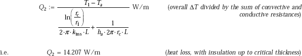
Therefore, percentage increase in heat dissipation:
Increase in current carrying capacity due to insulation:
Now, heat dissipation with bare wire, Q1 = I12 × R, and,
where, I1 and I2 are currents for bare wire and wire with insulation, respectively, and R is the electrical resistance of the wire. Therefore,
And,
Increase in current carrying capacity is given by:
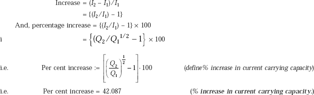
4.14 Optimum (or Economic) Thickness of Insulation
As mentioned earlier, insulation on a hot or cold surface reduces the heat loss and thus effects a considerable saving in energy. Therefore, choice of suitable insulation, its application to the surface and maintenance over the lifetime of insulation are very important aspects in industry.
Consider the case of an insulation being applied on a hot surface. As the thickness of insulation goes on increasing, the amount of heat loss from the surface goes on decreasing, i.e. the cost of energy lost goes on decreasing; but, at the same time, the first cost of material and labour to apply the insulation goes on increasing. Therefore, there are two opposing factors coming into consideration while determining the combined cost, namely, increased saving in cost of fuel (or energy) lost and increased expenditure for material and labour towards the insulation.
‘Optimum’ or ‘Economic’ thickness of insulation is that thickness for which the combined cost of the amount of energy lost through the insulation and the total (material + labour) cost of insulation is a minimum.
Obviously, optimum thickness of insulation depends on many factors: fixed cost such as material cost of insulation, and varying costs such as: cost of energy, interest and depreciation, taxes, maintenance costs, etc.
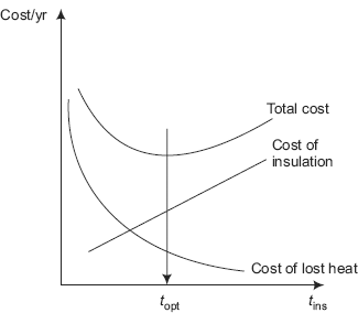
FIGURE 4.16(a) Determination of optimum thickness of insulation
Fig. 4.16 (a) shows cost of heat loss, cost of insulation and the total cost on an annualised basis, plotted against thickness of insulation:
From the figure we note that the cost of insulation increases with thickness almost linearly, whereas the cost of heat lost through insulation decreases exponentially. So, the total cost, which is the sum of these two costs, decreases initially, reaches a minimum and then increases again. Thickness at which total cost is a minimum is the optimum thickness. Mathematically, this is found out by differentiating the expression for total cost w.r.t. thickness and equating to zero.
If we wish to compare three or four insulations for the same job, we can draw similar ‘Total cost curves’ for those insulations and the thickness of the insulation having the lowest total cost is the optimum thickness. This is shown in Fig. 4.16 (b), where insulation D has optimum thickness.
Generally, optimum thickness of insulation is calculated in one of the following ways:
- Combined cost of heat lost plus the insulation (including material) on an yearly basis should be minimum, or
- The insulation should pay for itself in two or three years, i.e. the cost of material and labour of insulation should be equal to the cost of energy saved (by way of reducing the heat lost through the insulation) over two or three years, or
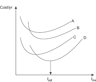
FIGURE 4.16(b) Comparison of insulations
- (iii) Minimise the total present cost, considering an interest rate, but neglecting other factors such as depreciation, taxes and maintenance costs.
In method (iii) mentioned above, the procedure to find optimum thickness of insulation is as follows:
Let Q be the heat loss through the insulation per year. Let Ch be the cost of heat loss per unit (Rs/kJ). So, the cost of heat loss/year = Q.Ch. Then, if i is the compound interest rate, compounded annually, the total present value of heat loss, P1 over the service life of n years is given by:
And, let the present material + labour cost for insulation be Clns Rs/m3. Then, if the volume of insulation applied is V (m3), the present value of insulation, P2 is given by:
Total present value or cost , PT is given by:
In Eq. c, first term on the RHS is dependent on radius (or thickness, L for a slab) of insulation, and by differentiating PT w.r.t. radius (or L) and equating to zero, we obtain the value of r (or L) that gives minimum PT. And then, optimum thickness is easily calculated.
Following examples illustrate the procedure of finding out the optimum thickness:
Example 4.22. A reactor, heated with saturated steam at 7.917 bar (Tsa t = 170°C) is 1.5 m in diameter and 2 m long, operates 5840 hrs per year. Assume that surface of the reactor is at 170°C and the ambient is at 30°C. It is insulated with an insulation of k = 0.038 W/(mC) which costs Rs. 16,000 per m3 of insulation (including cost of material, labour, cladding, etc.). Heat transfer coefficient on the outer surface is 30 W/(m2C). Cost of steam is Rs. 700 per ton. Latent heat of steam at the given conditions is 2050 kJ/kg. Efficiency of the steam heating may be taken as 80%. Determine the optimum thickness of insulation and the money saved per year. Assume that surface temperature of the reactor and the heat transfer coefficient remain the same for the reactor with and without insulation.
Solution.
Data:
D := 1.5 m L := 2 m T1 := 170°C Ta := 30°C ha := 30 W/(m2C) kins := 0.038 W/(mC)

First, we find out the cost of heat lost for the bare reactor (= Cost1). Then, for the insulated reactor, find the costs of energy lost through the insulation (i.e. CostP1) and the cost of insulation itself (i.e. CostP2) as a function of insulation thickness. Adding them together gives total cost (i.e. CostTotal). Find out the thickness at which the CostTotal is minimum by differentiating the expression for CostTotal and equating to zero, or graphically. This thickness is the ‘optimum thickness of insulation’. Now, find cost of heat lost through this insulation of optimum thickness per year (= Cost2).
Cost of heat lost from the surface of bare reactor (Cost1):
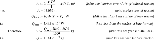
Efficiency of steam heating is 80%. Therefore, to dissipate Q amount of energy, the oven must consume an energy Qin = Q/0.8
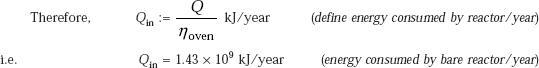
Now, find annual cost for bare reactor from the given data that 1 kJ costs Rs. 3.41463 × 10⁻⁴.
Cost 1 := Qin·Ch Rs/year |
(define annual cost of heat for bare reactor) |
Cost 1 := 4.884 × 10⁵ Rs/year |
(annual cost of heat for bare reactor.) |
Cost of heat loss through insulation, when reactor is insulated (CostP1):
When insulation is installed, the heat loss is determined from:
Further, since the reactor diameter is large (more than 1 m), we assume the surface to be flat, i.e. we will consider it as a slab to calculate the thermal resistance.
Let tins be the thickness of insulation.
Then, we can write:
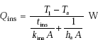
And, now, heat loss per year for furnace with insulation will be,
Efficiency of steam heating is 80%. Therefore, to dissipate Q1 amount of energy, the reactor must consume an energy Q1in = Q1/0.8, kJ/yr.
Now, find annual cost of heat loss for insulated reactor as a function of tins from the given data that 1 kJ costs Rs. 3.41463 × 10⁻⁴
Therefore,
Cost of insulation (material + labour etc.)…(i.e. CostP2):
Cost of insulation = Volume of insulation × cost per unit volume
i.e. CostP2(tins) := (A × tins) × Cins Rs
Therefore,
Total cost of (heat loss through insulation/yr + insulation)…(i.e. CostTotal):
To find optimum thickness of insulation…(i.e. topt):
Differentiate the expression for CostTotal w.r.t. tins and equate to zero. Root of the resulting equation is the value of topt.
In Mathcad, this procedure is very easy: First, assume a trial value of tins. Next, define the derivative of CostTotal as: CostTotal’. Then, use the ‘root function’ to find the root of CostTotal ’ = 0:
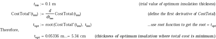
To fid topt graphically:
Plot the three costs, namely, CostP1, CostP2 and CostTotal as a function of tins. Optimum thickness is that thickness at which the CostTotal is a minimum.: This is very easily done in Mathcad: First, define a range variable tins varying from an initial value of say, 1 cm up to a final value of say, 20 cm with an increment of 0.5 cm. Then, select the x-y graph from the graph palette and fill in tins in the place holder on the x-axis. On the y-axis place holder, fill in CostP1(tins), CostP2 (tins), CostTotal (tins). Click outside the graph area and the three graphs appear immediately: See Fig. Ex. 4.22.
tins := 0.01, 0.015… 0.2 |
(define range variable tins: first value = 0.01 m, next value = 0.015 m and last value = 0.2 m) |
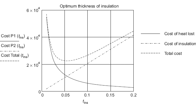
FIGURE Example 4.22
Note: Observe from the graph that the minimum of CostTotal is at 0.053 m, i.e. the optimum thickness of insulation = 0.053 m, as obtained mathmatically earlier.
Money saved per year due to insulation:
For the bare reactor, cost of heat lost from the surface per year is Cost1.
For the insulated reactor, insulated with optimum thickness of insulation, cost of heat lost per year is: CostP1(topt). Difference between these two costs is the money saved per year:
Cost1 = 4.884 × 10⁵ Rs |
(already calculated) |
CostP1(topt) = 1.133 × 10⁴ Rs/yr |
(cost of heat lost through optimum thickness of insulation) |
Saving per year is given by:
Therefore,
|
Saving := Cost1 − CostP1 (topt) |
(define Saving…money saved per year due to insulation) |
i.e. |
Saving = 4.771 × 10⁵ Rs/yr |
(money saved due to insulation.) |
It may be noted that method of finding out ‘optimum thickness’ of insulation is rather involved. In practice, it is more convenient to select the optimum thickness of insulation from the charts and tables prepared by TIMA (Thermal Insulation Manufacturers’ Association) and their member companies.
4.15 Effect of Variable Thermal Conductivity
In the cases considered so far, we assumed thermal conductivity, k to be constant, i.e. k did not change with temperature. However, this assumption may not be always true. When the k of a material varies rapidly with temperature or when the temperature range of operation is large, it becomes necessary to take into account the variation of k with temperature.
In general, analysis of heat transfer with variable k is complicated. However, for the special case of one-dimensional steady state heat conduction with no internal heat generation, solutions for simple geometries such as slabs, cylinders and spheres are obtained quite easily as explained below.
Generally, k varies with temperature linearly as follows:
where, |
ko = thermal conductivity at 0 deg. C |
|
β = temperature coefficient of thermal conductivity |
|
T = temperature above 0 deg. C. |
4.15.1 Plane Slab with Variable Thermal Conductivity
Consider a plane slab as shown in Fig. 4.17. Let the thickness be L. k is a linear function of temperature, given by Eq. 4.67. Temperatures at the two faces are constant and uniform, i.e. T = T1 at x = 0 and T = T2 at x = L.
Assumptions:
- One-dimensional conduction, i.e. thickness L is small compared to the dimensions in the y and z-directions
- Steady state conduction, i.e. temperature at any point within the slab does not change with time; of course, temperatures at different points within the slab will be different.
- No internal heat generation
- k varies linearly with temperature, i.e. k(T) = ko(1 + βT).
Our problem is to first, find out the temperature field within the slab and then, the heat flux at any point.
For the above assumptions, the governing differential equation reduces to:
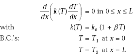
Solution to the above governing equation with the B.C.’s shown, gives the temperature profile and then, by applying Fourier’s law we can get the heat flux any point.
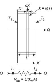
FIGURE 4.17 Plane slab with k = k(T) and the thermal circuit
Alternative, simple method:
For heat transfer rate, Q:
Remember that as far as there is steady state, one-dimensional heat transfer with no internal heat generation, Q flowing through each layer is a constant, as a consequence of First law. Then, we can directly integrate the Fourier’s equation. keeping the Q outside the integral sign, since it is a constant, though its value is yet unknown. Performing the integration within the limits of B.C.’s given, gets the value of Q. Then, using the fact that Q is the same between any two layers, we get the temperature profile. This method is outlined below:
Consider a differential element of thickness dx at a distance x from the origin as shown in Fig. 4.17. If dT is the temperature differential across this element, then we can write from Fourier’s law:
where, |
k(T) is given by Eq. 4.67 |
|
A = area normal to the direction of heat flow (same at all sections for a slab) |
Substituting for k(T), separating the variables and integrating from x = 0 to x = L (with T = T1 to T = T2), we get:
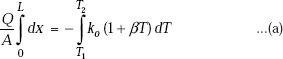
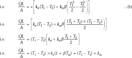
where, km = ko (1 + βTm) is the mean value of k at the mean value of temperature, Tm.
And, Tm = (T1 + T2)/2
Therefore,
Eq. c gives the heat transfer rate for the plane slab, with variable thermal conductivity, k varying linearly with temperature.
Eq. c is important since in most of the practical cases of insulation for furnaces or lagging of hot pipes, thermal conductivity, indeed, varies linearly with temperature.
Writing Eq. c in a form analogous to Ohm’s law:
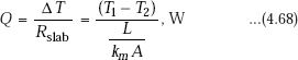
From Eq. 4.68, it is clear that expression for Q for a slab with thermal conductivity varying linearly with temperature, is of the same form as for a slab with constant k, except that k is replaced by km.
To get temperature distribution within the slab:
In Eq. a above, integrate between x = 0 and x = x (with correspondingly, T = T1 and T = T(x)), i.e. result is easily obtained by replacing L by x, T2 by T(x) in Eq. b:
We write from from Eq. b:
Equate Eqs. d and e, since in steady state, Q is same through each layer of the slab. We get:
Eq. f is a quadratic equation in T, whose roots are given by:
where,
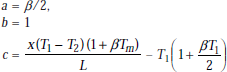
Therefore,
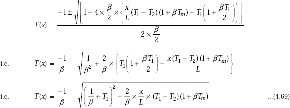
Eq. 4.69 gives the temperature distribution within the slab, with the thermal conductivity varying linearly with temperature.
Temperature profile is shown graphically in Fig. 4.18:
Note that: |
for β > 0, temperature profile is convex |
|
for β < 0, temperature profile is concave , and |
|
for β = 0, temperature profile is linear (i.e. for constant k, temperature profile is linear, as already shown). |
Shape of the temperature profile can easily be deduced as follows: From k = ko (1 + βT), we can write:
Therefore, for positive value of β: dk/dT is positive, i.e. k increases with increasing temperature or decreases with decreasing temperature. Now, from Fourier’s law:
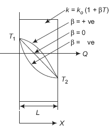
FIGURE 4.18 Temperature profile in a slab with variable k
As x increases, T decreases and, therefore, k also decreases. Then, to keep the heat flux, (Q/A), constant, –(dT/dx) must increase; i.e. (dT/dx) must decrease. So, the curve is convex. See the upper curve for β > 0 in Fig. 4.18.
For negative value of β, by similar argument, the curve will be concave as shown in Fig. 4.18.
Example 4.23. A plane wall of fire clay brick of thickness 25 cm has temperatures of 1350°C and 50°C on its two sides. k for fireclay brick varies as:
k(T) = 0.838 (1 + 0.0007 T), W/(mC) where T is in deg.C. Calculate:
- the rate of heat flow
- temperature at mid-plane
- distance of the plane at 400°C from LHS
- sketch the temperature distribution in the wall.
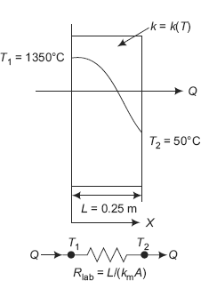
FIGURE Example 4.23 Plane wall—k varying linearly with T
Solution. See Fig. Ex. 4.23.
Data:
T1 := 1350°C T2 := 50°C L := 0.25 m A := 1 m2 k(T) := 0.838· (1 + 0.0007·T) W/(mC)
Note that k varies linearly with temperature since the above relation is of the form:
k(T) = ko(1 + βT), where: |
|
ko := 0.838 |
(k value at zero deg.C) |
β := 0.0007 |
(temperature coefficient conductivity) |
Since k is varying linearly with temperature, Q, the heat transfer rate is determined by the same formula as for plane slab with constant k, except that instead of k we have to use km, the mean value of k(T). Remember that for a plane slab with constant k, we have:
So, first, determine Tm = (T1 + T2)/2, then, km and then, Rsla b
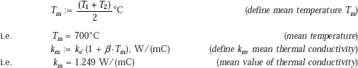
Thermal resistance:
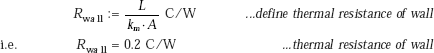
Heat transfer rate, Q:
Therefore,
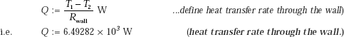
Temperature at mid-plane, i.e. at x = 0.125 m:
We can use Eq. 4.69 and substitute x = 0.125 in that equation.
However, let us work this out from fundamentals. Remember Q is same through each layer in steady state, since there is no internal heat generation. And, Q is already worked out to be 6492.82 W.
From Fourier’s law, at any x, we can write:
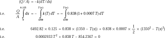
Solving for root of this quadratic equation in T, we get the value of T at x = 0.125 m, i.e. at mid-plane:
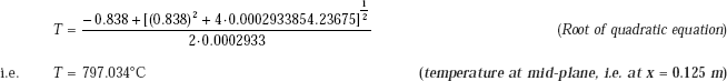
Verify: verify this value of T from direct formula 4.69:
We have:
Put x = 0.125
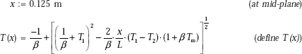
Therefore,
T(0.125) = 797.033°C (temperature at mid-plane…verified)
Note the ease with which Eq. 4.69 is evaluated in Mathcad.
Distance of the plane at 400°C from LHS:
Again, in Mathcad, we can solve this easily by Eq. 4.69. But, first let us solve it by conventional method: Let the distance of the plane at 400°C from origin (i.e. LHS) be x. Then,
Form Fourier’law, at any x, we can write:
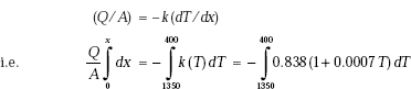
Here, Q is known, already calculated to be 6492.82 W; and, A = 1 m2 Performing the integration:
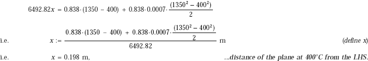
Verify: verify this value of x from direct formula 4.69:
We use the solve block. Start with a trial value of x. Put the constraint of Eq. 4.69 with T(x) as 400°C, immediately below ‘Given’. Then, the command ‘Find (x) =’ gives the value of x:
Given
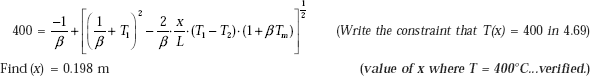
To draw temperature profile inside the wall:
Mathcad is ideally suited to do this. First, define a range variable x varying from 0 to 0.25 m, at an interval of 0.01 m. Then, select x - y graph from the graph palette, fill in x in the place holder on the x-axis and fill in T(x) in the place holder on y-axis. Click anywhere outside the graph, and immediately the graph is drawn: See Fig. Ex. 4.23(b).
x := 0, 0.01, …, 0.25 |
…define a range variable x, with starting value = 0, next value = 0.01 and last value = 0.25 m |
It may be verified from the above graph that temperatures at x = 0.125 m (i.e. mid-plane) and at x = 0.198 m are 797°C and 400°C, respectively.
Example 4.24. In a furnace, the gas temperature is maintained at 1300°C and the surrounding temperature is 30°C. The furnace walls are made of a layer of refractory material of thickness 30 cm and thermal conductivity k1 = (0.28 + 0.23324 × 10⁻³ T), W/(mC) and a layer of bricks with a thermal conductivity k2 = (0.113 + 0.023278 × 10⁻³ T), W/(mC). The heat transfer coefficient from gases to refractory wall is 30 W/(m2C) and that from brick to surroundings is 10 W/(m2C). What should be the thickness of brick layer of the setting so that the loss of heat to surroundings should not exceed 750 W/m2?
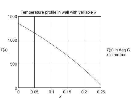
FIGURE Example 4.23(b)
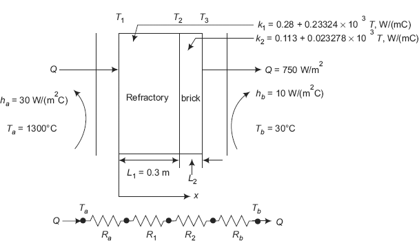
FIGURE Example 4.24 Furnace with insulations of variable k
Solution. See Fig. Example 4.24.
Data:
Ta := 1300°C (temperature of hot gases in furnace) Tb := 30°C(temperature of surroundings)
L1 := 0.3 m(thickness of refractory material)
Let L2 be the thickness of brick layer.
k1 : = 0.28 + 0.2334 × 10⁻³·T W(mC) (Thermal conductivity of refractory material)
k2 := 0.113 + 0.023278 × 10⁻³·T W(mC) ha := 30 W(mC) hb := 10 W(m2C) Q := 750 Wm2 A := 1 m2
This is the case of steady state, one-dimensional conduction with no internal heat generation in the walls. Therefore, thermal resistance concept is applicable. Also, use the fact that in steady state, heat flow rate through each layer is the same.
Fig. Example 4.24 shows the set up.
First, find temperatures T1 and T3, temperatures of exposed surfaces of refractory and the brick wall, respectively.
Convective thermal resistances Ra and Rb:
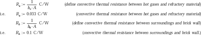
Temperatures T1 and T3:
Apply the fact that heat flow rate, Q, through both convective layers is the same, i.e. Q = 750 W/m2. Therefore, from Q = (Ta – T1)/Ra and Q = (T3 – Tb)/Rb, we write
|
T1 = Ta − Q.Ra, and |
|
|
T2 = Tb + Q.Rb |
|
|
T1 := Ta − Q.Ra°C |
(define T1, temperature of exposed surface of refractory layer) |
i.e. |
T1 = 1.275 × 10³°C |
(temperature of exposed surface of refractory layer.) |
|
T3 := Tb + Q·Rb°C |
(define T3, temperature of exposed surface of brick layer) |
i.e. |
T3 = 105°C |
(temperature of exposed surface of brick layer.) |
To find the interface temperature T2, between the two layers:
Apply the fact that Q through the refractory layer is 750 W/m2. Here, we note that thermal conductivity varies linearly. So, expression for the thermal resistance is the same as for a wall with constant thermal conductivity [i.e. R = L/(kA)] except that k is replaced by km.
So, R1 = L1/(kmA); km is obtained by substituting T = Tm = (T1 + T2)/2 in the given expression for k(T). Since T2 is not yet known, let us write:
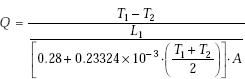
In the above equation, all values except T2 are known. So, simplifying, we get a quadratic equation in T2 and by solving that equation we get T2. This is left as an exercise to the student.
Instead of following that laborious procedure, let us use the solve block of Mathcad to solve for T2 easily:
Start with a trial value for T2 (say = T2 = 100) and write the above mentioned constraint immediately below ‘Given’. Then, the command ‘Find(T2) = ‘ instantly gives the value of T2:
Given
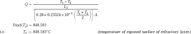
Thickness of the brick layer, L2:
Thickness of brick layer L2 is obtained by aplying the equivalent Ohm’s law to the brick layer, i.e. Q = ΔT/R2, where
R2 = thermal resistance of brick layer = L2/(km A); now, mean value of thermal conductivity, km has to be used since the thermal conductivity of brick layer varies linearly with temperature.
First, calculate km. For this, substitute the value of Tm in the given expression for k of brick layer. Tm = (T2 + T3)/2:
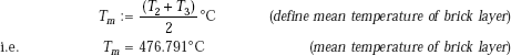
Therefore, mean value of thermal conductivity for brick layer is given by:
|
km := 0.113 + 0.023278 × 10⁻³·Tm W/(mC) |
(define mean temperature of brick layer) |
i.e. |
km = 1.124 W/(mC) |
(mean thermal conductivity of brick layer) |
Now, applying equivalent Ohm’s law to the brick layer:
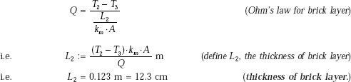
Example 4.25. Thermal conductivity of a plane wall varies with temperature according to the relation k(T) = ko (1 + β T2), where ko and β are constants.
- Develop an expression for the heat flow through the slab per unit area if the surfaces at x = 0 and x = L are maintained at uniform temperatures T1 and T2. respectively.
- Develop a relation for the thermal resistance of the wall if the heat transfer surface is A
- Calculate the heat transfer rate through A = 0.1 m2 of the plate for T1 = 200°C, T2 = 0°C, L = 0.4 m, k0 = 60 W/ (mC), and β = 0.25 × 10⁻⁴ C–2.
Solution. (a) Expression for heat transfer rate, Q:
First of all, note that in this case, thermal conductivity varies with temperature in a non-linear fashion; therefore, the relations derived earlier for mean thermal conductivity, km and thermal resistance, R, cannot be used.
However, still, it is a fact that there is one dimensional, steady state conduction with no heat generation in the wall. Therefore, from First law, Q, the heat transfer rate is same through any section of the slab. So, we can directly integrate Fourier’s equation, taking the Q outside the integral:
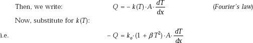
Separating the variables and integrating from x = 0 to x = L, (and T = T1 to T = T2),
we get:
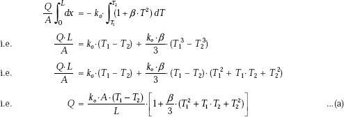
Eq. a is the required expression for the heat transfer rate, Q.
(b) Expression for thermal resistance:
Let us write Eq. a in the form analogous to the Ohm’s law:
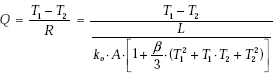
Therefore, it is clear that the thermal resistance is given by
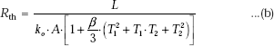
Eq. b gives the expression for thermal resistance for the wall with k varying with temperature as: k(T) = ko(1 + β T2).
(c) Numerical problem:
Data:
A := 0.1 m2 T1 := 200°C T2 := 0.0°C L := 0.4 m k0 := 60 W/(mC) β := 0.25 × 10⁻⁴ C–2
Therefore, heat transfer rate is given by Eq. a derived above:
Substituting the values and simplifying, we get:
4.15.2 Hollow Cylinder with Variable Thermal Conductivity
Consider a long, hollow cylinder as shown in Fig. 4.19. Let length of cylinder be L, inside radius ri and outside radius ro. Inner and outer surfaces are at uniform temperatures of Ti and To, respectively. Let k vary linearly with temperature as given by Eq. 4.67.
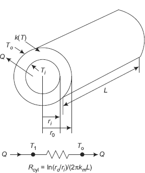
FIGURE 4.19(a) Cylindrical system with variable k and the equivalent thermal circuit
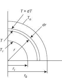
FIGURE 4.19(b) Elemental volume of thickness dr
Assumptions:
- Steady state conduction
- One-dimensional conduction, in the r direction only
- Thermal conductivity varies linearly with temperature
i.e. k(T) = ko(1 + βT)
- No internal heat generation.
Now, since this is a cylindrical system, we start with the general differential equation for one-dimensional conduction, in cylindrical coordinates (see Eq. 3.17). For the stipulated conditions, the governing equation reduces to:
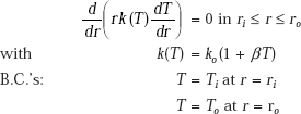
Solution to the above governing equation with the B.C.’s shown, gives the temperature profile and then, by applying Fourier’s law we can get the heat flux any point.
Alternatively:
For heat transfer rate, Q:
Since there is steady state, one-dimensional heat transfer with no internal heat generation, Q flowing through each layer is a constant, as a consequence of First law. Then, we can directly integrate the Fourier’s equation keeping Q outside the integral sign, since it is a constant, though its value is yet unknown. Performing the integration within the limits of B.C.’s given, gets the value of Q. Then, using the fact that Q is the same between any two layers, we get the temperature profile. This method is outlined below:
Consider a differential element of thickness dr at a distance r from the origin as shown in Fig. 4.19. If dT is the temperature differential across this element, then we can write from Fourier’s law:
where, |
k(T) is given by Eq. 4.67 |
|
Ar = area at radius r, normal to the direction of heat flow = 2πrL |
|
dT/dr is the temperature gradient |
Substituting for k(T), separating the variables and integrating from r = ri to r = ro (with T = Ti to T = To), we get:
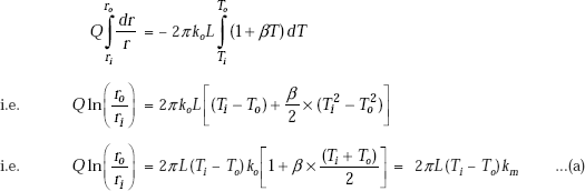
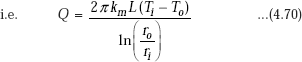
where,
km |
= ko(1 + β Tm) = mean value of thermal conductivity and, |
Tm |
= (Ti + To)/2 = mean value of temperature. |
Note that Eq. 4.70 for heat transfer Q for a cylindrical system with linearly varying k, is of the same as form as for a cylindrical system with constant k, except that k is replaced by km.
Eq. 4.70 is important since in most of the practical cases of insulation for lagging of hot pipes, thermal conductivity, indeed, varies linearly with temperature.
Writing Eq. 4.70 in a form analogous to Ohm’s law, i.e. Q = ΔT/R, it is clear that thermal resistance of a cylindrical system with linearly varying k is given by:
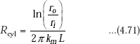
To get temperature distribution within the cylindrical shell:
Integrate the Fourier’s equation. between r = ri and r = r. (with correspondingly, T = Ti and T = T(r)), i.e. result is easily obtained by replacing ro by r, To by T(r) in Eq. a:
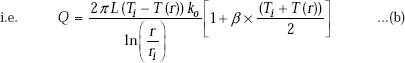
We write from Eq. a:
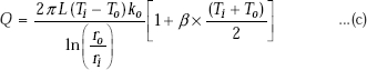
Equate Eqs. b and c, since in steady state, Q is the same through each layer of the cylinder:
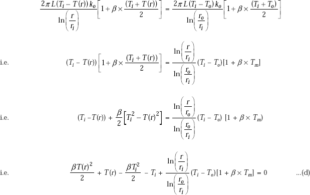
Eq. d is a quadratic in T(r). Its roots are given by:
where, |
a = β/2, |
|
b = 1 |
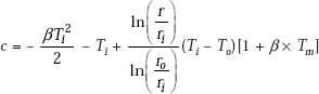
Therefore,
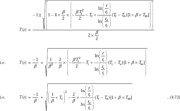
Eq. 4.72 gives the temperature distribution within the cylindrical shell, with the thermal conductivity varying linearly with temperature.
Compare this with Eq. 4.69 for a slab with the k varying linearly with temperature.
Example 4.26. The inner and outer radii of a hollow cylinder are 5 and 10 cm, respectively. The inside surface is maintained at 300°C and the outside surface at 100°C. The thermal conductivity varies with temperature over this temperature range as: k(T) = 0.5 × (1 + 10–3 T), where T is in deg.C and k(T) is in W/(mC). Determine:
- heat flow rate per metre length of cylinder
- temperature at mid-thickness of shell, and
- sketch the temperature profile within the shell.
Solution. See Fig. Ex. 4.26.
Data:
ri := 0.05 m |
ro := 0.10 m |
L := 1 m |
Ti := 300°C |
To := 100°C |
k(T) := 0.5·(1 + 10–3·T) |
Therefore, comparing with k(T) = ko (1 + βT), we write:
ko := 0.5 W/(mC) |
(k at zero deg.C) |
β := 10−3 C−1 |
(temperature coefficient of thermal conductivity.) |
Recognise immediately that the thermal conductivity varies with temperature linearly.
Therefore, expression for the heat transfer rate, Q, for a cylindrical shell is of the same form as that for the case of constant k, except that k is replaced by km, the mean value of thermal conductivity. See Eq. 4.70.
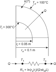
FIGURE Example 4.26 Cylinder with variable k and equivalent thermal circuit
Heat transfer rate, Q:
First, find Tm and then, km. Then use Eq. 4.70:
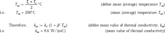
Therefore,
Thermal resistance:
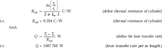
Temperature at mid-thickness of shell, i.e. at r = 0.075 m:
This can be found out directly from Eq. (4.72) by substituting r = 0.075. But, let us first work this out from fundamentals and then verify the result from Eq. 4.72. If T is the temperature at r, then use the fact that Q is the same through each layer of the shell. Remember, Q is already calculated above.
From Fourier’s equation, we have:
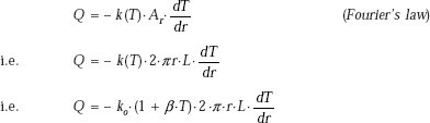
Separating the variables and integrating from r = r1 to r = r (and T = T1 to T = T) and keeping Q outside the integral, since it is a constant):
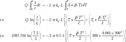
Simplifying, we get:
This is a quadratic equation in T, whose positive root is:
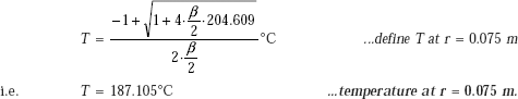
The above procedure is the conventional procedure where you get the quadratic equation in T and then, solve for its roots. However, when you use Mathcad, there is no need for all that labour; just use the solve block of Mathcad. Start with a trial value of T (say, 120°C) and in the solve block, immediately below ‘Given’, write the constraint, given by Eq. a above. There is no need to perform the integration, since Mathcad does it internally. Then, the command ‘Find(T) =’ immediately gives the value of T:
r := 0.075 m |
(radius at mid-thickness) |
T := 120°C |
(trial value of temperature at r = 0.075 m) |
Given
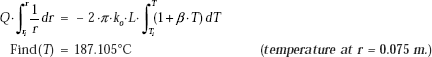
Verify: Now, verify this result from Eq. 4.72:
Rewriting Eq. 4.72:
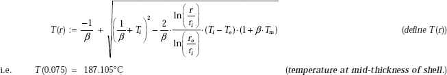
To sketch the temperature distribution in the shell:
First, define the range variable, r, varying from r = 0.05 m to r = 0.1 m, with an increment of 0.001 m. Then, choose the x – y graph from the graph palette, fill in ’r and ‘T(r)’ in the place holders on the x-axis and y-axis respectively. Click anywhere outside the graph region and immediately the graph appears:
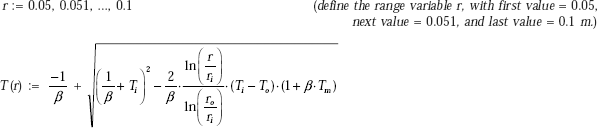
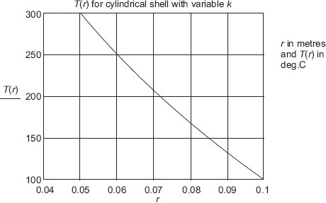
FIGURE Example 4.26(b)
It may be seen from the graph that at the inside and outside surfaces of the cylindrical shell, the temperatures are 100°C and 300°C, respectively, as given in data.
Example 4.27. A steam pipe, 20 cm OD carries steam at 260°C and is insulated with a material whose thermal conductivity varies linearly with temperature. Insulation thickness is 6 cm. Outer surface of insulation is at 60°C and the heat flow rate in steady state is measured to be 230 W/m. Reported value of k for this insulation is 0.081 W/(mC) at 100°C. Find out the expression for k(T). Also, find the temperature at mid-thickness of insulation and sketch the temperature profile in the insulation.
Solution.
Data.
ri := 0.10 m r0 := 0.16 m L := 1 m Ti := 260°C T0 := 60°C Q := 230 W/m
Since it is given that the thermal conductivity varies with temperature linearly, expression for the heat transfer rate, Q, for a cylindrical shell is of the same form as that for the case of constant k, except that k is replaced by km, the mean value of thermal conductivity. See Eq. 4.70.
From Eq. 4.70, we have:
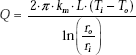
Therefore,
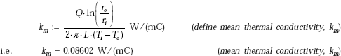
Now, for linear variation of k with T, we have the variation of the form:
Here, use ko = 0.081 W/(mC) and for T substitute (T – 100):
Therefore,
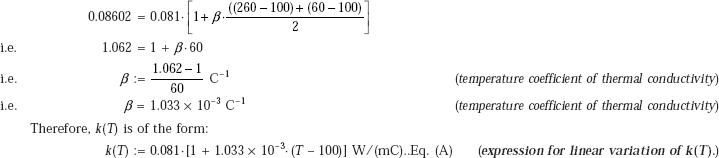
Temperature at mid-thickness, i.e. at r = 0.13 m:
Temperature at r = 0.13 m is calculated by integrating Fourier’s equation from r = r1 to r = r (and T = T1 to T = T). While doing so, Q is constant and can, therefore, be taken out of the integral sign:
From Fourier’s equation we have:
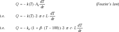
Separating the variables and integrating from r = ri to r = r (and T = Ti to T = T) and keeping Q outside the integral, since it is a constant):
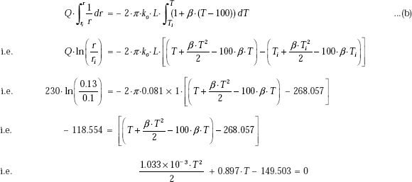
This is a quadratic equation in T, whose positive root is given by:
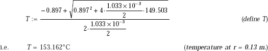
Note: Above-mentioned procedure is, however, laborious. Instead, let us solve for T using solve block of Mathcad. Start with a trial value of T (say, 100°C) and in the solve block, immediately below ‘Given’, write the constraint, given by Eq. (B). Then, the command ‘Find(T) = ‘immediately gives the value of T; But, we will define T (r) = Find(T), so that the same solve block will repeatedly calculate T for any r. This will be useful to draw the temperature profile, i.e. T(r) vs. r.
r := 0.13 m |
(value of r at mid-thickness of insulation) |
T := 100°C |
(trial value of temperature at radius r) |
Given
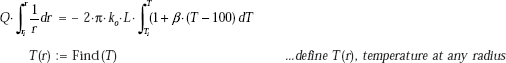
Therefore,
T(0.13) = 153.197°C |
(Temperature at r = 0.13 m.) |
Once again, note the great advantage of using the solve block. For any r, now the temperature T(r) can be calculated by just putting the value of r in T(r). This will be used to sketch the temperature profile in the insulation:
To sketch the temperature profile in the insulation:
This is done easily in Mathcad. First, define a range variable r, varying from r = 0.1 m to r = 0.16 m, with an increment of 0.001 m. Then choose x-y graph from the graph palette and fill in the place holders on the x-axis and y-axis with ‘r’ and ‘T (r)’, respectively. Click anywhere outside the graph region and immediately the graph appears: See. Fig. Ex. 4.27.
r := 0.1, 0.101, …, 0.16 |
(define the range variable r, with first value = 0.1, next value = 0.101, and last value = 0.16 m.) |
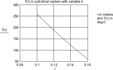
FIGURE Example 4.27
Check: check the value of T(0.13) obtained above by finding out the value of Q between r = 0.1 m and r = 0.13 m; Since Q should be the same through each layer, we should get Q = 230 W: Between r = 0.1 m (Ti = 260°C) and r = 0.13 m (T = 153.197°C), find km and then apply Eq. 4.70:
From Eq. A:

Then, from Eq. 4.70:
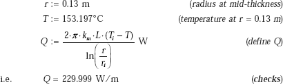
4.15.3 Hollow Sphere with Variable Thermal Conductivity
Consider a hollow sphere as shown in Fig. 4.20. Let the inside radius be ri and outside radius ro. Inner and outer surfaces are at uniform temperatures of Ti and To, respectively. (Ti > To). Let k of the material vary with linearly with temperature as given by Eq. 4.67 i.e. k (T) = ko (1 + βT).
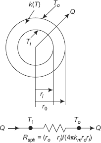
FIGURE 4.20(a) Spherical system with variable k and the equivalent thermal circuit
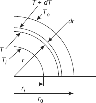
FIGURE 4.20(b) Elemental volume of thickness dr
Assumptions:
- Steady state conduction
- One-dimensional conduction, in the r direction only
- Thermal conductivity varies linearly with temperature, i.e. k(T) = ko (1 + βT)
- No internal heat generation.
Now, since this is a spherical system, we start with the general differential equation for one dimensional conduction, in spherical coordinates (see Eq. 3.21). For the stipulated conditions, the governing equation reduces to:
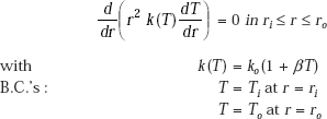
Solution to the above governing equation with the B.C.’s shown, gives the temperature profile and then, by applying Fourier’s law we can get the heat flux any point.
Alternatively:
For heat transfer rate, Q:
Since there is steady state, one-dimensional heat transfer with no internal heat generation, Q flowing through each layer of the spherical shell is a constant, as a consequence of First law. Then, we can directly integrate the Fourier’s equation keeping the Q outside the integral sign, since it is a constant, though its value is yet unknown. Performing the integration within the limits of B.C.’s given, we get the value of Q. Then, using the fact that Q is the same between any two layers, we get the temperature profile. This method is outlined below:
Consider a differential element of thickness dr at a distance r from the origin as shown in Fig. 4.20. If dT is the temperature differential across this element, then we can write from Fourier’s law:
where, |
k(T) is given by Eq. 4.67 |
|
Ar = area at radius r, normal to the direction of heat flow = 4 πr2 |
|
dT/dr is the temperature gradient |
Substituting for k(T), separating the variables and integrating from r = ri to r = ro (with T = Ti to T = To), we get:
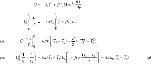
where,
ko = km(1 + β Tm) = mean value of thermal conductivity and,
Tm = (Ti + To)/2 = mean value of temperature
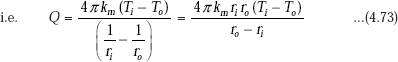
Note that Eq. 4.73 for heat transfer Q for a spherical system with linearly varying k, is of the same as form as for a spherical system with constant k, except that k is replaced by km.
Eq. 4.73 is important since in most of the practical cases, thermal conductivity varies linearly with temperature. Writing Eq. 4.73 in a form analogous to Ohm’s law, i.e. Q = ΔT/R, it is clear that thermal resistance of a spherical system with linearly varying k is given by:
To get temperature distribution within the spherical shell:
Integrate the Fourier’s equation between r = ri and r = r (with correspondingly, T = Ti and T = T(r)), i.e. result is easily obtained by replacing ro by r, To by T(r) in Eq. a:
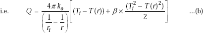
We write from Eq. a:
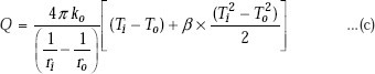
Equate Eqs. b and c, since in steady state, Q is the same through each layer of the sphere. Simplifying, we get a quadratic equation in T(r). Its solution gives the value of T(r), the temperature at radius r. This is left as an exercise to the student.
Final expression for T(r) is:

Eq. 4.75 gives the temperature distribution within the spherical shell, with the thermal conductivity varying linearly with temperature. Compare this with Eq. 4.69 for a slab, and 4.72 for a cylinder, with the k varying linearly with temperature.
Example 4.28. The inside and outside surfaces of a hollow sphere, a < r < b, at r = a and r = b are maintained at uniform temperatures T1 and T2, respectively. The thermal conductivity varies with temperature as:
- Develop an expression for the total heat flow rate Q through the sphere.
- Develop a relation for the thermal resistance of the hollow sphere.
Solution. Note that now, the variation of k with temperature is not linear; however, the method to solve the problem is the same as adopted earlier, i.e. consider an elemental volume of thickness dr and directly integrate the Fourier’s equation from r = a to r = b, remembering that in steady state, one-dimensional conduction, with no internal heat generation, Q is the same through each layer and is, therefore, taken out of the integral sign.
See Fig. Example 4.28.
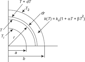
FIGURE Example 4.28 Sphere with non-linear variation of k(T)
So, for an elemental volume at a radius r and of thickness dr, we have:
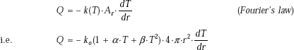
Separating the variables and integrating from r = a to r = b (and corresponding, T = T1 to T = T2), we get:
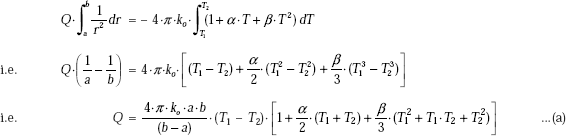
Eq. a is the desired expression for heat transfer rate, Q.
Thermal resistance:
Writing Eq. a in a form analogous to Ohm’s law, i.e. Q = ΔT/R, we get:
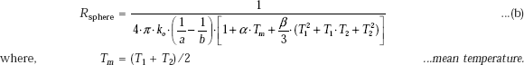
Eq. b gives the required expression for thermal resistance of the sphere with temperature dependent k.
Example 4.29. An insulated spherical container to store liquid nitrogen, is overall 0.5 m OD and the insulation is 12 cm thick, whose k varies with temperature as:
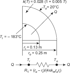
FIGURE Example 4.29 Sphere with variable k
If surface temperature of the sphere is 90 K, and the outside surface is at 20°C, find out:
- heat transfer rate in steady state
- temperature at mid-thickness of insulation, and
- sketch the temperature profile.
Solution. See Fig. Ex. 4.29
Recognise immediately that the thermal conductivity varies with temperature linearly.
Therefore, expression for the heat transfer rate, Q, for a spherical shell is of the same form as that for the case of constant k, except that k is replaced by km, the mean value of thermal conductivity. See Eq. 4.73.
Data:
ri := 0.13 m ro := 0.25 m Ti := – 183°C To := 20°C k(T) := 0.028·(1 + 5 × 10⁻³·T)
Therefore, comparing with k(T) = ko(1 + βT), we write: ko := 0.028 W/(mC) β := 5 × 10⁻³ C–1
Heat transfer rate, Q:
First, find Tm and then, km. Then use Eq. 4.73:
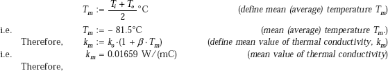
Thermal resistance:
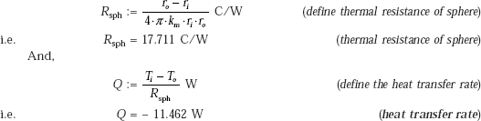
Note: Negative value of Q indicates that heat transfer is from outside to inside (i.e. in the direction opposite to the positive r direction).
Temperature at mid-thickness of shell i.e. at r = 0.19 m:
This can be found out directly from Eq. 4.75 by substituting r = 0.075.
But, let us first work this out from fundamentals and then verify the result from Eq. 4.75.
If T is the temperature at r, then use the fact that Q is the same through each layer of the shell. Remember, Q is already calculated above.
From Fourier’ equation, we have:
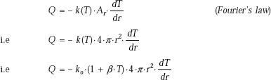
Separating the variables and integrating from r = r1 to r = r (and T = Ti to T = T) and keeping Q outside the integral, since it is a constant):
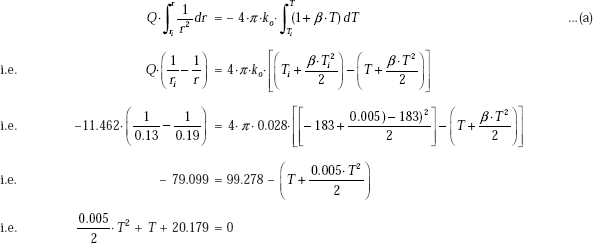
This is a quadratic equation in T, whose root is
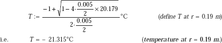
Note: When we use Mathcad, there is no need to adopt the above tedious procedure. Instead, use the solve block. Start with a trial value of T (say, 10°C) and in the solve block, immediately below ‘Given’, write the constraint, given by Eq. a above. There is no need to perform the integration, since Mathcad does it internally. Then, the command ‘Find(T) =’ immediately gives the value of T:
r := 0.19 m |
(radius at mid-thickness of shell) |
T := 10°C |
(trial value of T) |
Given
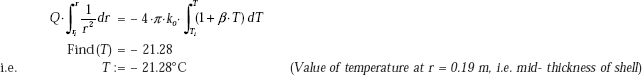
Verify: Now, verify this result from Eq. 4.75 too: Rewriting Eq. 4.75:
Rewriting Eq. 4.75:

To sketch the temperature distribution in the shell:
First, define the range variable, r, varying from r = 0.13 m to r = 0.25 m, with an increment of 0.001 m. Then, choose the x-y graph from the graph palette, fill in ’r and Temp(r) in the place holders on the x-axis and y-axis respectively. Click anywhere outside the graph region and immediately the graph appears:
r := 0.13, 0.131, …, 0.25 |
(define range variable r, with first value = 0.13 m, next value = 0.131 m, and last value = 0.25 m) |
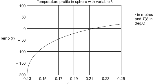
FIGURE Example 4.29(b)
Note how the temperature within the spherical insulation shell increases from –183°C at r = 0.13 m to 20°C at r = 0.25 m; temperature at mid-thickness (r = 0.19 m) is – 21.28°C, as calculated earlier.
4.16 Two-dimensional Conduction—Shape Factor
So far, we have considered heat transfer in different geometries assuming that heat transfer is one-dimensional. This is a very good approximation and gives closely accurate results for simple geometries such as slabs, cylinders and spheres. However, there are many practical cases where this is not a reality as in the case of irregular shapes or when the temperatures along the boundaries are non-uniform. In such cases, heat transfer will be in more than one-dimension. Practical examples are: heat treatment of engineering components of irregular shapes, heat transfer in I.C. engine blocks, chimneys, air conditioning ducts, etc.
To solve multidimensional heat transfer problems, basically, there are four methods:
Analytical method. In this method start with the general differential equation for conduction in the required coordinate system and solve it in conjunction with the given initial and boundary conditions to get the temperature field; then apply the Fourier’s equation and get the heat flux at any desired point. However, this method is suitable only to simple geometries. Otherwise, the solutions are quite cumbersome and require knowledge of infinite series, Bessel functions, Legendre polynomials, Laplace transform methods and complex variable theory.
Graphical method. Graphical methods are used for two-dimensional problems with isothermal and adiabatic boundaries. This is an approximate method. Here, temperature and heat flow lines are drawn by free hand, remembering that isothermal and heat flow lines are orthogonal, thus forming curvilinear squares. Once such a ‘flux plot’ is drawn, heat flow is easily calculated by applying Fourier’s law to each ‘heat flow lane’. Again, this method is suitable to simple geometries only and was popular in the early days when computing techniques were primitive. This method is now almost obsolete.
Analogical method. This method makes use of the electrical analogy between the governing equations of electrostatics and heat conduction to plot the potential field:
i.e.
and,
i.e. temperature and voltage are analogous.
Special conducting paper (or, conducting solution in a bath) is used to make a model of the geometry being investigated and the isothermal (equipotential) lines are traced using a probe. Then, heat flow lines are drawn normal to the isothermal lines. This method is more accurate than free hand plotting.
Numerical method. Here, the body is divided into a number of discrete sub-volumes; centre of each sub-volume is called a ‘node’ and the nodes are connected by fictitious ‘conducting rods’. By making a heat balance on each node a set of algebraic equations are obtained and these are solved by standard methods to get the temperature field.
Of the above-mentioned methods, numerical methods have taken over other methods because of availability of high speed computers and the ability to analyse complex shapes and deal with complicated boundary conditions. We shall explain this technique in a later chapter.
Shape factors for two-dimensional conduction:
Here, we will explain an approximate, but simple method to analyse a particular type of 2-D conduction problems where steady state heat transfer occurs between two surfaces at fixed temperatures, T1 and T2, with an intervening solid medium in between. If Q is the rate of heat transfer between two temperature potentials T1 and T2, with the thermal conductivity of intervening material being k, with no heat generation in the medium, we write:
where, S is known as shape factor and has dimension of length. Note that Eq. 4.76 is applicable only when there is conduction, i.e. in solids. For liquids and gases, where convection is generally the predominant phenomenon, this equation is not applicable.
From Eq. 4.76, immediately it follows that thermal resistance of the medium is given by:
Now, recall that thermal resistance of a plane wall, cylinder and sphere are given, respectively, by:
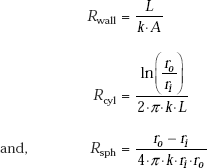
From this, since we can write: S = 1/(R.k), we get:
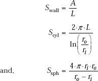
One important application of the concept of shape factor is in calculation of heat transfer in a furnace. Here, separate shape factors are used to calculate the heat flow through the walls, edges and corners. When all the interior dimensions are greater than one-fifth of the wall thickness, we get:
where, A = inside area of the wall, L = wall thickness, and D = length of edge.
S has been computed by researchers using electrical analogy or numerical methods, for several cases of practical interest.
Figs. 4.21 to 4.30 give conduction shape factors for a few selected two-dimensional systems:
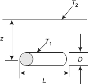
FIGURE 4.21
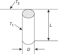
FIGURE 4.22
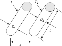
FIGURE 4.23
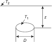
FIGURE 4.24
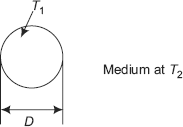
FIGURE 4.25
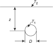
FIGURE 4.26
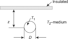
FIGURE 4.27
A square flow passage
For a/b > 1.4: |
S = 2πL/{0.93 ln (0.948 a/b)} |
For a/b < 1.41: |
S = 2πL/{0.785 ln(a/b)} |
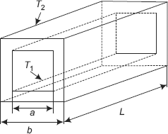
FIGURE 4.28
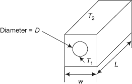
FIGURE 4.29
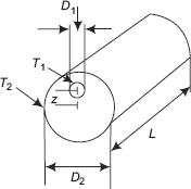
FIGURE 4.30
Example 4.30. A spherical tank of diameter D = 2 m containing radio-active material is buried in the earth. The distance between earth’s surface and the tank’s centre is 5 m. Heat release resulting from radioactive decay in the tank is 700 W. Calculate the steady state temperature of tank’s surface if the earth’s surface is at 10°C. The value of k of earth at this location may be taken as: k = 1 W/(mC).
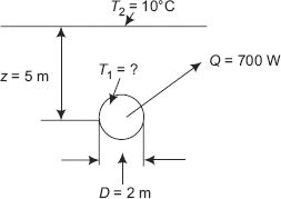
FIGURE Example 4.30 Isothermal sphere buried in a semi-infinite medium
Solution. Refer to Fig. Example 4.30.
Data:
D := 2 m z := 5 m T2 := 10°C Q := 700 W k := 1 W(mC)
For this situation, Shape factor is given in Fig. 4.26.
We have:
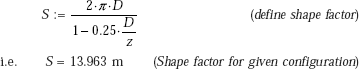
Also,Q= k·S·(T1 – T2) where T1 is the temperature of tank’s surface.
Therefore,
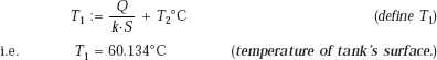
Example 4.31. Inside dimensions of a small cubical furnace constructed of fireclay bricks (k = 1.04 W/ (mC)) are: 0.6 m × 0.6 m × 0.6 m, walls being 0.1 m thick. The temperatures on the inside and outside surfaces are 550°C and 50°C, respectively. Determine the heat lost from the furnace.
Solution. Recognise that this problem can be solved by use of ‘shape factors’. Also, recall that when the interior dimensions of the furnace are greater than one-fifth of the wall thickness, we have, for Shape factors:
where, A = inside area of the wall, L = wall thickness, and D = length of edge.
See Fig. Example 4.31.
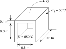
FIGURE Example 4.31 Cubical furnace
Note that for a cubical structure, there are 6 wall sections, 12 edges and 8 corners. Calculate the Shape factors and compute the total Shape factor by adding all of them.
Data:
Size of furnace: 0.6 m × 0.6 m, × 0.6 m i.e. dimension of each wall, D = 0.6 m
D := 0.6 m L := 0.1 m A := D·D m2
i.e. A = 0.36 m2 k := 1.04 W/(mC) T1 := 550°C T2 := 50°C
S for Walls:
S for a single wall section is given by:
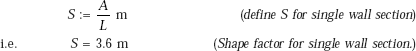
Therefore, for 6 wall sections:
|
Swalls := S·6 m |
(S for 6 wall sections) |
i.e. |
Swalls = 21.6 m |
(S for 6 wall sections) |
S for Edges:
S for a single edge is given by:
|
S := 0.54·D m |
(define S for single edge) |
i.e. |
S = 0.324 m |
(Shape factor for single edge.) |
Therefore, for 12 edges:
|
Sedges := S·12 m |
(S for 12 edges) |
i.e. |
Sedges = 3.888 m |
(S for 12 edges) |
S for Corners:
S for a single corner is given by:
|
S := 0.15·L m |
(define S for single corner) |
i.e. |
S = 0.015 m |
(Shape factor for single corner.) |
Therefore, for 8 corners:
|
Scorners := S·8 m |
(S for 8 corners) |
i.e. |
Scorners = 0.12 m |
(S for 8 corners) |
Total Shape factor:
Therefore, total shape factor is obtained by summing up the shape factors for all the walls, edges and corners:
|
Stotal := Swalls + Sedges + Scorners m |
(total shape factor) |
i.e. |
Stotal = 25.608 m |
(total shape factor) |
Heat transfer rate, Q:
Therefore, total heat loss from the furnace is given by:
|
Q := k·Stotal·(T1 − T2), W |
(define Q) |
i.e. |
Q = 1.332 × 10⁴ W = 13.32 kW |
(total heat loss rate from furnace.) |
4.17 Summary of Basic Conduction Relations
We have analysed steady state, one-dimensional heat transfer, with no internal heat generation, in three important geometries, namely, plane slab, cylinder and sphere and derived relations for temperature distribution and rate of heat transfer. We also studied the effect of variable thermal conductivity on these results. Since all these relations are practically important, they are tabulated in Table 4.4 and Table 4.5, for easy reference.
TABLE 4.4 Relations for steady state, one-dimensional conduction with no internal heat generation, and constant k
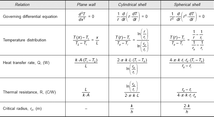
TABLE 4.5(a) Relations for steady state, one-dimensional conduction with no internal heat generation and k varying linearly with temperature as:
k(T) = ko(1 + βT)
km = ko(1 + βTm); Tm = (T1 + T2)/2
| Relation | Plane wall |
|---|---|
Governing differential equation |
|
Temperature distribution, T(x) |
|
Heat transfer rate, Q, (W) |
|
Thermal resistance, R, (C/W) |
|
TABLE 4.5(b) Relations for steady state, one-dimensional conduction with no internal heat generation, and k varying linearly with temperature as:
k(T) = ko(1 + βT)
km = ko(1 + βTm); Tm = (Ti + To)/2
| Relation | Cylindrical shell |
|---|---|
Governing differential equation |
|
Temperature distribution, T(r) |
|
Heat transfer rate, Q, (W) |
|
Thermal resistance, R, (C/W) |
|
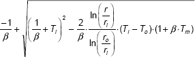
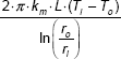

TABLE 4.5(c) Relations for steady state, one-dimensional conduction with no internal heat generation, and k varying linearly with temperature as:
k(T) = ko(1 + βT)
km = ko(1 + βTm); Tm = (Ti + To)/2
| Relation | Spherical shell |
|---|---|
Governing differential equation |
|
Temperature distribution, T(r) |
|
Heat transfer rate, Q, (W) |
|
Thermal resistance, R, (C/W) |
|
4.18 Summary
In this chapter, we studied the application of general differential equation for conduction to the cases of steady state, one-dimensional conduction, with no internal heat generation, in three simple, but important geometries, namely, plane slab, cylinder and sphere. Expressions for temperature distribution and rate of heat transfer were derived in these cases by two approaches:
- starting with the appropriate differential equation for the problem under consideration, and
- by direct integration of Fourier’s equation.
Despite the mathematical simplicity of the relations derived, note that these relations give reasonably accurate results in practical situations.
Concept of thermal resistance was used to solve steady state, one-dimensional heat transfer problems in composite systems with no internal heat generation. Concept of contact resistance, and how to include its effect on heat transfer rate was explained.
Critical radius of insulation was studied for cylindrical and spherical systems; how to find out the optimum thickness of insulation was also indicated.
Next, the effect variable conductivity on rate of heat transfer and temperature distribution was explained with reference to the above-mentioned three geometries.
Finally, different methods of solving multi-dimensional heat transfer problems were briefly mentioned and Shape factors for two-dimensional heat transfer for many cases of practical importance were tabulated.
In the next chapter, we shall continue the study of steady state, one-dimensional heat conduction in simple geometries, but with internal heat generation.
Questions
- Explain what is meant by ‘one-dimensional conduction’.
- Explain ‘log mean area’ for a hollow cylindrical system and ‘geometric mean area’ for a hollow spherical system.
[M.U.]
- Explain the concept of ‘thermal resistance’. What are its applications?
- Derive an expression to determine the heat flow through a composite cylindrical shell with two layers. Assume no heat generation and that steady state is reached.
[M.U.]
- Derive the following expression for loss of heat from a lagged pipe per square metre of metal surface per degree temperature difference between the metal and lagging surface:

where, k is the thermal conductivity of lagging material; r and R are the radii of metal and lagging surface. Neglect thermal resistance due to metal surface.
[V.T.U.]
- Derive an expression for steady state heat transfer through a composite spherical shell with two layers.
[M.U.]
- Prove that steady state heat transfer rate through the walls of spherical container is given by:
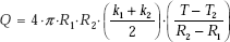
where, k = k1 + (k2 – k1) (T – T1)/(T2 – T1) and T1, T2, k1, k2,, R1, R2 are all constants.
[M.U.]
- Show that the heat transfer in a steady state unidirectional conduction through a spherical wall is given by:
Q = πkd1d2 ΔT/δ
where, d1 and d2 are the inner and outer diameter of the sphere, respectively and δ is the wall thickness.
[M.U.]
- What do you mean by ‘overall heat transfer coefficient’? Derive an expression for the same for the case of a composite cylinder of two layers, based on inside surface as well as outside surface (i.e. for Ui and Uo)
- Derive an expression for critical thickness of insulation in case of an electric cable. Explain the significance of critical thickness.
[V.T.U.]
- Show that for a sphere, critical radius is given by: rc = 2 kins/h.
- The thermal conductivity of a certain material varies according to the following relation: k = k0(1+αT), where k0 and α are constants. Prove that the heat transfer at steady state condition through a plane wall of thickness L is given by
Q = kmA (T1 – T2)/L
where, km = ko[1 + α (T1 + T2)/2]
Also, derive the equation for temperature distribution.
[M.U.]
- Steady one-dimensional heat conduction takes place through the slab of a material whose thermal conductivity varies linearly with T as: k(T) = k0(1 + aT) where a is a constant. The slab is of thickness s and the two faces of the slab are maintained at temperatures T1 and T2. There is no heat generation within the slab. Solving basic differential equation for one-dimensional, steady state conduction, find out the expression for temperature distribution within the slab.
[M.U.]
- When thermal conductivity varies linearly with T as: k(T) = k0 (1 + βT), show that heat transfer rate through a cylindrical shell is given by:

All notations have usual meaning.
- When thermal conductivity varies linearly with T as: k(T) = k0(1 + βT), show that heat transfer rate through a spherical shell is given by:
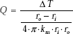
All notations have usual meaning.
- A spherical shell of radii r1 and r2 is made of material with thermal conductivity k(T) = k0T2. Derive an expression for the heat transfer rate if the surfaces are held at temperatures T1 and T2, respectively.
[M.U.]
- What do you mean by ‘optimum thickness’ of insulation? How is it determined?
- Enumerate different methods of solving two-dimensional heat conduction problems.
- What is ‘conduction shape factor’? How is it related to thermal resistance? Explain its applications.
Problems
Plane slabs and composite slabs:
1. A brick wall (k = 0.7 W/(mC)) is 0.3 m thick. Inner surface is maintained at 45°C and outside surface, at 25°C. Calculate the heat transfer rate per m2 of area. Also, find the temperature at the mid-plane.
2. A large window glass of thickness 4 mm (k = 0.78 W/(mC)) is exposed to warm air at 20°C at its inner surface, with a convective heat transfer coefficient between inner surface and air being 15 W/(m2C). Outside air is at –10°C and associated heat transfer coefficient is 45 W/(m2C). Find out the temperatures of inner and outer surfaces of the glass and the overall heat transfer coefficient.
3. A furnace wall is made up of 12 cm thick fireclay (k = 0.93 W/(mK)), 20 cm thick red brick (k = 0.7 W/(mK)) with covering of 6 mm thick mild steel plate (k = 39 W(mK)). 18 steel bolts, each of 20 mm diameter are used per m2 for fixing the steel plate and composite wall together. Find the heat transfer per m2 of furnace wall (length of bolt 32.6 cm).
[M.U.]
4. A house wall may be approximated as two 1.2 cm layers of fibre insulating board, a 8 cm layer of loosely packed asbestos and a 10 cm layer of common brick. Assuming convection heat transfer coefficients of 15 W/(m2K) on both sides of the wall, calculate the overall heat transfer coefficient for this arrangement. (kfibre board = 0.033 W/ (mK), kasbestos = 0.17 W/(mK), kbrick = 0.65 W/(mK).
[M.U.]
5. A composite wall consists of 15 cm thick layer of material A and a 30 cm thick layer of material B. Thermal conductivity of the two materials are different and unknown but constant. The outer surface temperature of material A is 250°C and the outer surface temperature of material B is 50°C. An insulation of k = 0.05 W/(mK) and thickness 2 cm is added to the outer face of B. It is observed that outer surface of A acquires a temperature of 330°C and the junction between B and insulation is at 230°C. The outer surface of insulation is at 30°C. Estimate the rate of heat flow per m2.
- before the addition of insulation.
- after the addition of insulation.
[M.U.]
6. A furnace wall 30 cm thick has k = 1.4 W/(mK). The heat transfer coefficient of the outer surface is given as h = (8.1 + 0.09. ΔT) where ΔT is the temperature difference between outside wall surface and surrounding. If the inner surface temperature is 1450°C, calculate the rate of heat loss per unit area. The furnace wall is insulated such that the heat losses do not exceed 500 W/m2. This is done by putting two layers of insulation on the outer surface; the first one is of heat resisting brick of k = 0.6 W/(mK) and the second one is of silica brick of k = 0.15 W/(mK). If the thickness of silica brick is 30 cm, find the thickness of heat resisting brick. Assume the surrounding temperature as 40°C.
[M.U]
7. The inside temperature of furnace wall, 200 mm thick, is 1350°C. The mean thermal conductivity of wall material is 1.35 W/(mC). The heat transfer coefficient of outside surface is a function of temperature difference and is given by: h = 7.85 + 0.08 ΔT where ΔT is the temperature difference between outside wall surface and surroundings. Determine the rate of heat transfer per unit area, if the surrounding temp. is 40°C.
[M.U.]
8.
- Calculate the rate of heat flow through 1 m2 area of a clean heating surface of a steam boiler if the flue gas temperature is 1500°C and the boiling water temperature is 250°C. The heat transfer coefficients from gas to the wall and from the wall to the water are 120 W/(m2C) and 4500 W/(m2C) m respectively. The thermal conductivity of boiler wall material is 52 W/(mC) and its thickness is 12 mm.
- If the heating surface exposed to the gas side is covered with soot layer of 1 mm (k = 0.07 W/(mC)) and water side surface is covered with scale of 1.5 mm thickness (k = 0.8 W/(mC)), calculate the rate of heat flow and surface temperatures of the corresponding layers.
[M.U.]
9. In order to reduce heat loss from a furnace wall, the thickness of its brickwork is increased by 100%. The temperature of the inner surface of the brickwork is 660°C. The temperature of the outer surface, before increasing the wall thickness was 235°C. Calculate the percentage decrease in the heat loss due to increase in brickwork thickness. Assume that the thermal conductivity and heat transfer coefficient remain constant. Take atmospheric temperature as 35°C.
[M.U.]
10. A furnace wall is made of composite wall of total thickness 55 cm. The inside layer is made of refractory material of k = 2.3 W/(mK) and the outside layer is made of an insulating material of k = 0.2 W/(mK). The mean temperature of the gases inside furnace is 900°C and the interface temperature is 520°C. The heat transfer coefficient between the gases and inner surface can be taken as 230 W/(m2K) and between outer surface and atmosphere as 46 W/(m2K). Assuming the temperature of surrounding air as 30°C, calculate:
- required thickness of each layer
- rate of heat loss per unit area, and
- the temperature of the surface exposed to gases and of the surface exposed to atmosphere.
[M.U.]
Contact resistance:
11. A plane composite wall is made of two materials A and B with thermal conductivities kA = 0.1 W(mK) and kB = 0.04 W/(mK). Thicknesses are LA = 10 mm and LB = 20 mm. Contact resistance between the layers is 5 × 10⁻⁴ m2K/W. A fluid at 400°C flows over the free surface area of A with ha = 12 W/(m2K) and a fluid at 30°C flows over the surface of B with hb = 25 W/ (m2K). Determine the rate of heat transfer per m2 of the wall surface, temperature drop at the interface and overall heat transfer coefficient.
12. Two 5 cm diameter, 15 cm long aluminium bars (k = 176 W/(mC)), with ground surfaces are held against each other at a pressure of 20 bar and the thermal contact conductance at the interface, hc = 11,000 W/(m2C). Bars are insulated along their length. Top and bottom surfaces of this two-bar system are maintained at temperature of 250°C and 30°C, respectively. Calculate the rate of heat transfer along the bar in steady state and also the temperature drop at the interface.
Variable area:
13. Ends A and B of a tapered rod, 250 mm long are 50 mm and 25 mm in diameter. The rod is insulated along its lateral surface. If A and B are maintained at temperatures of 300°C and 27°C, respectively, and k of the material is 40 W/(mC), find, in steady state:
- heat flow rate through the rod, and
- temperature at mid-point.
14. Circular cross section of a cone like solid (k = 25 W/ (mK)), shown in Fig. Problem 4.14, varies as: D = 0.5 x0.5. x1 = 25 mm from origin and x2 = 125 mm. Temperatures T1 and T2 are maintained at 700 K and 500 K, respectively. Lateral surface is well-insulated.
Calculate:
- steady state heat transfer rate
- temperature at mid-section.
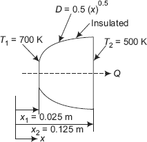
FIGURE Problem 4.14 Tapered cone-like solid
Cylinders and composite cylinders:
15. A steam pipe, 0.12 m OD is insulated with 25 mm thick layer of an insulation of k = 0.08 W/(mK). Temperature of inner and outer surfaces of the insulation are 400°C and 40°C, respectively. Find the steady state rate of heat loss per metre length of pipe. Also, find the temperature of insulation at its mid-thickness.
16. A stainless steel tube (k = 19 W/(mK)), 2 cm ID and 4 cm OD is covered with a 4 cm layer of asbestos insulation (k = 0.2 W/(mK)). If the steady state heat loss rate per metre length of tube is measured to be 750 W/m, and the outside surface temperature is limited to 50°C, what is the temperature of the inside wall of the tube?
17. A metal (k = 45 W/(mK)) steam pipe of 5 cm ID and 6.5 cm OD is lagged with 2.75 cm radial thickness of high temperature insulation having thermal conductivity of 1.1 W/(mK). hi and ho are 4650 W/(m2K) and 11.5 W/(m2K), respectively. If the steam temperature is 200°C and the ambient temperature is 25°C, calculate:
- heat loss per metre length of pipe
- temperatures at the interfaces
- overall coefficient of heat transfer referred to inside and outside surfaces (i.e. calculate Ui and Uo).
[M.U.]
18. A steel pipe having an external diameter of 8 cm carries steam at 40 bar and is lagged with a layer, 4 cm thick of material of k = 0.04 W/(mK). Ambient temperature is 20°C and the surface of lagging has h = 10 W/(m2K). What thickness of lagging of k = 0.06 W/(mK) must be added to reduce the steam condensation by 50% if the surface coefficient remains unchanged? Neglect resistance of the pipe material and also of the steam film on the inside of the steam pipe.
[M.U.]
19. A steam pipe (k = 45 W/(mK)) having 70 mm. I.D. and 85 mm O.D. is lagged with two insulation layers; the layer in contact with the pipe is 35 mm thick asbestos (k = 0.15 W/(mK)) and it is covered with 25 mm thick magnesia insulation (k = 0.075 W/(mK)). The heat transfer coefficients for inside and outside surfaces are 220 W/(m2K) and 6.5 W/(m2K) respectively. If the temperature of steam is 350°C and ambient temperature is 30°C, calculate: (i) the steady state heat loss per metre length of pipe. (ii) overall heat transfer coefficients based on: (a) inside surface of pipe, and (b) outside surface of pipe.
[M.U.]
20. A 200 mm ID pipe carries superheated steam at 210°C. The value of k of pipe material = 13 W/(mK). The outside insulating layer has k = 0.2 W/(mK). Mean temperature at the interface is 195°C. h between steam and pipe wall = 60 W/(m2K) and between outer surface and ambient air is 35 W/(m2K). Assuming the total thickness of pipe (including pipe material) is 100 mm, ambient air at 30°C, calculate:
- required thickness of each layer
- rate of heat transfer per unit outer area, and
- inner and outer surface temperatures.
Spheres and composite spheres:
21. A hollow sphere of 5 cm ID, 10 cm OD is made of a material of k = 45 W/(mC). What is the heat flux required at the inner surface to maintain a steady state, inside surface temperature of 200°C when the outside surface temperature is 15°C? What is the temperature at the mid-thickness of the shell?
22. A hollow sphere of 10 cm ID, 30 cm OD, of material k = 35 W/(mK), contains a liquid chemical. Inner and outer surface temperatures are 450°C and 150°C. Determine the heat flow rate through the sphere. Also, estimate the temperature at a point quarter of the way between the inner and outer surfaces.
23. A spherical tank, 1 m in diameter is maintained at temperature of 120°C and exposed to a convection environment with h = 25 W/(m2K) and temperature of ambient is 15°C. What thickness of urethane foam (k = 20 mW/ (mK)) should be added to ensure that the outer temperature of the insulation does not exceed 40°C? What percentage reduction in heat loss results from installing this insulation?
24. A hollow spherical form is used to determine thermal conductivity (k) of an insulator. It has an ID of 20 cm, OD of 50 cm. A heater located at the centre of the sphere dissipates 30 W in steady state operation. Under steady conditions, temperatures at radii of 15 cm and 20 cm were measured to be 80°C and 60°C, respectively. Determine the k. Also, find the outer surface temperature. If the surrounding is at 30°C, what is the heat transfer coefficient over the surface? Plot the temperature profile along the radius.
25. A 600 mm OD sphere storing liquid is provided with two insulating layers, a high temperature insulation of k = 0.35 W/(mK) and a low temperature insulation of k = 0.07 W/(mK). The thickness of the former is 100 mm. The temperature drop across the high temperature insulation is required to be 2.5 times that across the low temperature insulation. What should be the thickness of the latter?
[V.T.U.]
‘Critical radius’ and ‘optimum thickness’ of insulation:
26. Determine the critical radius for a pipe covered with a layer of asbestos (k = 0.2 W/(mC)), exposed to atmosphere, if the outside heat transfer coefficient is
27. An electrical conductor of diameter 1.5 mm is covered with an insulation of k = 0.15 W/(mC).
- If the external convective heat transfer coefficient is 40 W/(m2C), what is the thickness of insulation that will cause maximum heat transfer?
- If the surface of the conductor is maintained at 150°C and ambient temperature is 30°C, and convective heat transfer coefficient remains the same, what is the rate of heat transfer (i) for bare wire, and (ii) with optimum insulation?
28. A sphere of diameter 5 cm is heated electrically from inside. It is exposed to an ambient at 30°C with a heat transfer coefficient of 25 W/(m2C). If the surface of the sphere is to be maintained at 150°C, calculate the rate of heat loss from the sphere:
- if the sphere is bare
- if the sphere is covered with insulation of k = 1 W/(mC) to a thickness that will cause maximum heat transfer.
29. A hollow copper sphere has outer radius of 5 cm. The internal temperature gradient can be neglected. The temperature of the sphere is to be maintained at 100°C by an embedded electric heater. The surrounding temperature is 20°C and the outside heat transfer coefficient is 10 W/(m2K). If this sphere is covered by 5 cm thick insulation (k = 0.5 W/(mK)), what will happen to heat loss? Calculate the percentage change in heat loss.
[M.U.]
30. A 1 mm diameter wire is maintained at a temperature of 350°C and exposed to convective environment at 30°C with h = 120 W/(m2K). Calculate the thermal conductivity which will just cause an insulation thickness of 0.2 mm to produce a critical radius. How much of this insulation must be added to reduce the heat transfer to 75% of that which would be experienced by the bare wire?
31. An electric cable of 10 mm diameter is to be laid in the atmosphere at 25°C. The estimated surface temperature of the cable due to heat generation is 65°C. Find the maximum percentage increase in heat dissipated, when the wire is insulated with rubber of k = 0.16 W/(mK). Take h0 = 10 W/(m2K).
[M.U.]
32. A wire of 8 mm diameter at a temperature of 60°C is to be insulated by a material having k = 0.174 W/(mK). Given: h0 = 8 W/mK, ambient temperature = 25°C. For maximum heat loss, what is the minimum thickness of insulation and heat loss per metre length? Also, find the increase in heat dissipation due to insulation.
[M.U.]
33. A cylindrical vessel, heated with saturated steam at 6.18 bar (Tsat = 160°C) is 1.0 m in diameter and 1.6 m long, operates 16 hrs. per day, 365 days a year. Assume that surface of the reactor is at 160°C and the ambient is at 25°C. It is insulated with an insulation of k = 0.038 W/(mC) which costs Rs. 17,000 per m3 of insulation (including cost of material, labour, cladding, etc.). Heat transfer coefficient on the outer surface is 25 W/(m2C). Cost of steam is Rs. 750 per ton. Latent heat of steam at the given conditions is 2083 kJ/kg. Determine the optimum thickness of insulation and the money saved per year. Assume that surface temperature of the vessel and the heat transfer coefficient remain the same for the reactor with and without insulation.
34. A 85 mm diameter pipe will carry steam at 220°C. It is proposed to lag it with an insulation of k = 0.15 W/(mC) such that heat transfer rate is reduced to 25% of that from the bare pipe. The outside heat transfer coefficient with air for lagged pipe is 10 W/(m2C) and, that from the bare pipe at 220°C is 25 W/(m2C). The ambient temperature is 30°C. If the estimated insulation cost is Rs. 16,000/m3 (including installation and other expenses) and the steam cost is Rs. 800 per ton, calculate the pay-back period, assuming a rate of interest of Re. 0.18/ (yr)(Re). Latent heat of steam is 1859 kJ/kg.
Variable thermal conductivity (slabs, cylinders and spheres):
35. The wall of a furnace consists of two layers, one of fireclay of thickness 12.25 cm and the other of red brick of thickness 48 cm. The thermal conductivity of fireclay is a function of temperature and its given by k1 = (0.28 + 0.00023 T) W/(mK) where T is in degree Celsius. k2 = thermal conductivity of red brick =0.7 W/(mK). The inside surface temperature is 1150°C and outside red brick wall temperature is 55°C. Calculate the amount of heat lost per m2 area of the furnace wall and interface temperature.
[M.U.]
36. Thermal conductivity of a plane slab varies with temperature as: k(T) = k0(1 + βT2), where k0 and β are constants. If the slab is 0.3 m thick and k0 = 60 W/(mC), β = 0.25 × 10⁻⁴ C–2 and the two faces of the slab are maintained at 250°C and 30°C, respectively, find out the steady state heat transfer rate per m2 of the area. Also, calculate the temperature at mid-thickness. Plot the temperature profile along the thickness.
37. A hollow cylinder whose k varies with temperature as: k(T) = 0.5 (1 + 0.001 T), where T is in deg.C, has an ID of 7.5 cm and OD of 12.5 cm. If the inside and outside surfaces are at uniform temperatures of 250°C and 100°C, respectively, find out the steady state heat transfer rate per metre length of pipe. Also, find out the temperature at a radius of 10 cm.
38. A long, hollow cylinder is constructed from a material whose k varies with temperature as: k(T) = (0.01 + 0.001 T), where k(T) is in W/(mK) and T is in deg.C. The inner and outer radii of the cylinder are 125 mm and 250 mm respectively. Under steady state conditions, the inner and outer surface temperatures are 698 K and 363 K, respectively. Determine:
- the rate of heat flow per metre length
- the temperature of the air on the outside of the cylinder, if the surface heat transfer coefficient on the exterior surface is 14.5 W/(m2K).
[V.T.U.]
39. Thermal conductivity of a sphere, 6 cm ID, 10 cm OD, varies as: k(T) = k0(1 βT3), W/(mC), where T is in deg.C. Calculate the steady state heat transfer rate if k0 = 60 W/(mC), β = 0.25 × 10⁻⁴, C–3, and Ti = 200°C and T0 = 0°C. Also, calculate the temperature at mid-thickness. Plot the temperature along the radius.
40. A cylindrical pressure vessel of 1 m ID and wall thickness 15 cm has the thermal conductivity of its material varying as: k(T) = 44 × (1 – 0.00042 T), W/(mC) where T is in deg.C. If the inside surface temperature is 500°C and the outer surface temperature is 300°C, what is the steady state heat transfer rate? Also, calculate the temperature at mid-thickness. Plot the temperature variation along the radius.
41. A spherical vessel, 0.3 m ID and 12 cm thick, is made of a material with k(T) = 51 × (1 – 0.0008 T), W/(mK) where T is in deg.C. Inside surface is at – 160°C and outside surface at –50°C. Calculate the heat loss. What is the temperature at mid-thickness? Plot the temperature along the radius.
Conduction shape factors:
42. An isothermal sphere of radius r = 8 cm is buried in a large body of earth. The sphere is maintained at an uniform temperature of 150°C; temperature of earth at large distance from the sphere is 15°C. Calculate the rate of heat loss from the sphere, in steady state if k of earth is 1.2 W/(mC).
43. Two parallel pipes are buried in earth with a spacing of 0.5 m between their centre lines. One of the pipes has a radius r1 = 8 cm and its surface is at 80°C; the other pipe has a radius of r2 = 5 cm and its surface is at 200°C. Calculate the heat transfer rate between the pipes per metre length of pipes if k of earth is 1.2 W/(mC).
44. A sphere of 1 m OD containing a radioactive material is buried such that its upper-most point is 1.5 m below the earth’s surface. If the outside surface temperature of the sphere is 450°C and k of the soil is 1.2 W/(mC), determine the rate of heat loss from the sphere. Surface temperature of soil is 30°C.
45. Inside dimensions of a furnace are: 3 m × 2.5 m × 2 m and walls are 0.2 m thick, with a k = 1.3 W/(mC). Temperature of inner and outer surfaces are 400°C and 50°C, respectively. Calculate the rate of heat loss from the furnace.
Example 4.1. Consider a slab of thickness L = 0.3 m. One face of the slab is at 100°C and the other face is at 0°C. Determine the heat flux across this slab if the slab is made of:
- pure copper (k = 382. 5 W/(mC))
- pure aluminium (k = 204 W/mC)), and
- building brick (k = 0.69 W/mC))
Also calculate temperature at the midplane (i.e. at x = 0.15 m) for each case. Compare their thermal resistances.
Solution.
Data:
L |
= 0.3 m |
A |
= 1 m |
T1 |
= 100°C |
T2 |
= 0°C |
Case 1: Material: Copper
Heat flux, q:
Therefore,
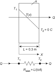
FIGURE Example 4.1
Temperature at mid-plane i.e. at x = 0.15 m:
Therefore,
T(0.15) = 50·C |
…Temperature at midplane |
T(0.1) = 66.667·C |
…Temperature at x = 0.1 m |
Thermal resistance, Rslab:
Therefore,
Case 2: Material: Aluminium
Heat flux, q:
Therefore,
Temperature at mid-plane i.e. at x = 0.15 m:
Therefore,
T(0.15) = 50°C |
…Temperature at midplane |
T(0.1) = 66.667°C |
…Temperature at x = 0.1 m |
Thermal resistance, Rslab
Therefore,
Case 3: Material: Building Brick
Heat flux, q:
Therefore,
Temperature at mid-plane i.e. at x = 0.15 m:
Therefore,
T(0.15) = 50°C |
…Temperature at midplane |
T(0.1) = 66.667°C |
…Temperature at x = 0.1 m |
Thermal resistance, Rslab
Therefore,
Note:
- Heat flux does not depend on x, but only on k, T1, T2 and L. Higher the value of thermal conductivity, higher the value of heat flux.
- Temperature at any point depends only on x and is independent of k
- Thermal resistance, Rslab = 0.00078843, 0.001471 and 0.435 C/W for copper, aluminium and building brick respectively; i.e. smaller the value of thermal conductivity, larger the value of thermal resistance. Obviously, insulators offer much higher resistance to heat flow as compared to metals.
Example 4.18. A hollow aluminium sphere (k = 200 W/(mC)), with inner radius rl = 0.15 m and outer radius r2 = 0.18 m is used to determine the thermal conductivity of an insulation material. Inner surface of aluminium is maintained at 250°C and 80 W is dissipated by the heater at the centre. The insulation material to be tested is cast on the outer surface of the sphere to a thickness of 0.12 m. This system is kept in a room at 20°C; convection coefficient ha between the outer surface of insulation and air is 30 W/(m2K). Find out the thermal conductivity of insulation. Also, find interface temperature T2 and outer surface temperature, T3.
Solution. Here, we have steady state, one-dimensional conduction with no internal heat generation in the layers. So, thermal resistance concept is applicable; also, heat transfer rate, Q, through each layer is the same.
Data:
r1 = 0.15 m |
…inner radius of aluminium sphere |
r2 = 0.18 m |
…outer radius of aluminium sphere |
r3 = 0.30 m |
…outer radius of insulation |
kAl = 200 W/(mC) |
…thermal conductivity of aluminium |
T1 = 250°C |
…temperature of inner surface of sphere |
Ta = 20°C |
…temperature of ambient air |
ha = 30 W/(m2K) |
…heat transfer coefficient between outer surface and air |
Q = 80 W |
…steady state heat dissipation |
Fig. Example. 4.18 shows the schematic and the equivalent thermal circuit.
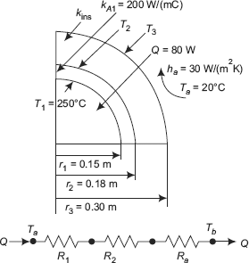
FIGURE Example 4.18 Composite spheres and equivalent thermal circuit
There are three thermal resistances, namely. conductive resistance of Al spherical shell (R1), conductive resistance of insulation spherical shell (R2) and convective resistance on the outer surface of insulation (Ra). R1 and Ra can be calculated, but we do not yet know kins to calculate R2. However, since Q is given, find out the total resistance, Rtot from Ohm’s law, i.e. Rtot = ΔT/Q. And, get R2 from R2 = Rtot – (Rl+Ra). Then, from expression for R2 (i.e. Eq. 4.55, get kins. Remember that total resistance, Rtot is found out by adding Rl, R2 and Ra, since they are all in series.
Temperature resistances:
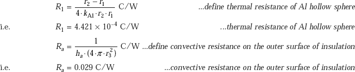
Total resistances, Rtot:
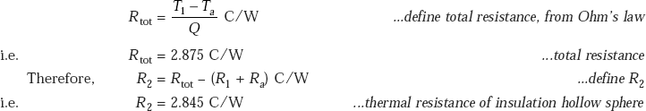
However, expression for R2 is given by Eq. (4.55):
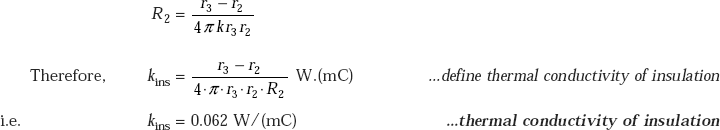
Interface temperature, T2:
Apply equivalent Ohm’s law to the Al shell:
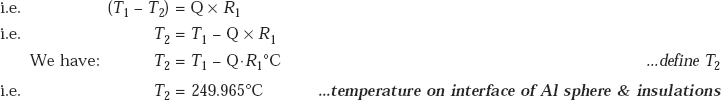
Note that temperature drop in Al shell is very small because of its very low thermal resistance.
Outer surface temperature, T3:
Apply equivalent Ohm’s law to the insulation shell:
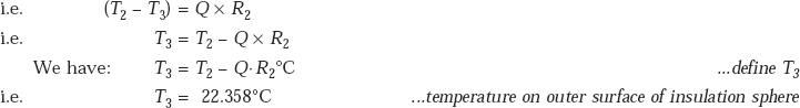
Check:
Apply equivalent Ohm’s law to the convection layer and verify that Q is same as 80 W:
Example 4.25. A 100 mm diameter pipe will carry steam at 160°C. It is proposed to lag it with 100 mm thick pre-formed insulation. The outside heat transfer coefficient with air for lagged pipe is 5 W/(m2C) and, that from the bare pipe at 160°C is 20 W/(m2C). Mean value of thermal conductivity of insulation is: km = 0.94 W/(mC), and the ambient temperature is 30°C. If the estimated insulation cost is Rs. 15000/m3 (including installation and other expenses) and the steam cost is Rs. 750 per ton, calculate the pay-back period, assuming a rate of interest of Re. 0.18/(yr) (Re). Latent heat of steam is 1825 kJ/kg.
Solution. See Fig. Example 4.25.
Data:
r1 = 0.05 m |
…outer radius of pipe |
r2 = 0.15 m |
…outer radius of lagging |
L = 1 m |
…length of pipe |
T1 = 160°C |
…surface temperature of furnace |
Ta = 30°C |
…ambient temperature |
ha1 = 20 W/(m2C) |
…heat transfer coefficient between bare pipe and ambient |
ha2 = 5 W/(m2C) |
…heat transfer coefficient between lagged pipe and ambient |
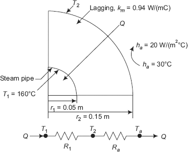
FIGURE Example 4.25(a) Steam pipe with lagging
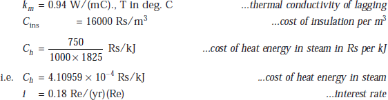
Let n years be the pay-back period.
First, we find out the cost of heat lost for the bare pipe (i.e. Cost1). Then, for the insulated pipe, find the cost of energy lost through the insulation (i.e. CostP1), compounded yearly with the given interest, over the service life (n years) of insulation. Difference between these two costs is the saving in energy due to insulation. This must be set equal to the cost of insulation itself (i.e. CostP2) and the resulting equation is solved to get the pay-back period, n.
Cost of heat lost from the surface of pipe (Cost1):
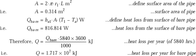
Now, find annual cost for bare pipe from the given data that 1 kJ costs Rs. 4.10959 × 10⁻⁴.
|
Cost1 = Q·Ch Rs/year |
…define annual cost of heat loss for bare pipe |
i.e. |
Cost1 = 7.057 × 10³ Rs/year |
…annual cost of heat loss for bare pipe |
Cost of heat loss through insulation, when pipe is insulated (CostP1):
When insulation is installed, the heat loss is determined from:
Since the pipe is cylindrical, Rcond is the thermal resistance for a cylindrical shell.
Rconv is convective thermal resistance over the surface of lagging.
Then, we can write:
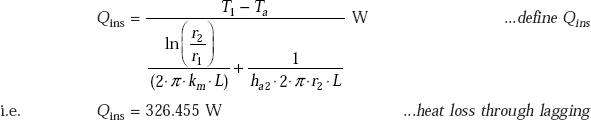
Therefore, cost of heat loos for one year is given by:
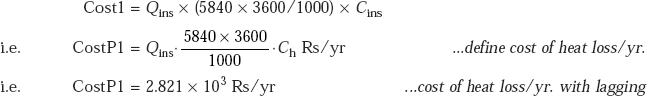
When i is the annual compound interest rate (compounded annually), total ‘present value’ of heat loss over a service period of n years is given by:
Therefore, saving in energy is given by the difference between Cost1 and PresentCostP1 i.e. Saving = Cost1 – PresentCostP1. Equate this to the cost of insulation.
Cost of insulation is given by:
i.e. we can write:
To find out the pay-back period:
To find out the pay-back period, n, let use Mathcad, since Mathcad does the required summation from 1 to n with ease. For this, click on the Summation symbol  from the Calculus palette and fill in the place holders as shown below.
Make a Table, each column showing: no. of years, n, PresntCostPl of lost heat through insulation over n years, and the Saving in Cost = [Costl – PresentCostPl].
Value of n when the last column is equal to CostP2 (i.e. cost of insulation), is the required service life or pay-back period.
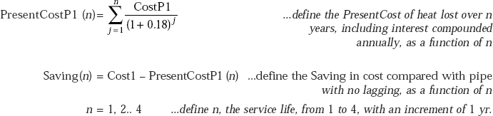
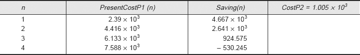
It may be observed that 3 years can be taken as the pay-back period since at n = 3, Saving value is about Rs. 925 and this is almost equal to Cost of insulation i.e. Rs. l005.
Again note: Cost of heat loss for bare pipe/yr. is Rs. 7,057.00, Cost of heat loss for lagged pipe, per yr. = Rs. 2,82l.00, and cost of insulation itself = Rs. l,005.00. Therefore, saving per yr because of use of lagging = (7057 – 282l) = 4236.00;
So, without considering any interest rate etc. the insulation pays for itself in about (4236/ l005) = about 4.2 yrs. Obviously, if we consider the interest rate also on saving, we can say that the insulation pays for itself in about 3 yrs.
Example 4.29. The two faces of a slab at x = 0 and x = L are kept at uniform temperatures Tl and T2, respectively, and the thermal conductivity of the material depends on temperature in the form k(T) = ko (T2 – To2), where ko and To are constants.
- Find an expression for the heat flow rate per unit area of the slab.
- Find an expression for the average thermal conductivity, km for the slab.
Solution. (a) Expression for heat transfer rate, Q:
Note that in this case too, thermal conductivity varies with temperature in a non-linear fashion; therefore, we proceed with direct integration of Fourier’s equation., taking Q outside the integral since it is a constant for stipulations of one-dimensional, steady state conduction with no heat generation in the wall:
Now, substitute for k(T):
i.e. ![]()
Separating the variables and integrating from x = 0 to x = L, (and T = T1 to T = T2), we get:
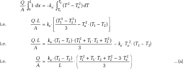
Eq. a is the required expression for the heat transfer rate per unit area, Q/A.
(b) Expression for average thermal conductivity km:
Let use write Eq. a in the form:
Then, comparing with Eq. a, it is clear that:
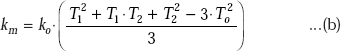
Eq. b is the required expression for average thermal conductivity, km.
Example 4.35. A pipe carrying a hot fluid (Tf = 150°C) is buried in earth. Distance between the pipe centre and earth’s surface is z = 1 m. The pipe has an OD of 20 cm and is covered with a 5 cm thick fibreglass insulation (k = 0.04 W/(mC)). The earth has a thermal conductivity k = 1.3 W/ (mC) and earth’s surface is at 0°C. Determine the heat loss per 10 m length of pipe. Also calculate the temperature of the outer surface of insulation.
Solution. This is a 2-D heat transfer problem; to be solved by using Shape factor. Shape factor for the given configuration is obtained from Fig. 4.21.
Remember:
The resistance to flow of heat from the cylinder consists of:
- conduction resistance through the cylindrical layer of fibreglass insulation, and
- thermal resistance of earth
In steady state, with no heat generation in either the fibreglass layer or the earth, Q is same through both these layers.
Data:
Let T1 be the outer surface temperature of fibreglass insulation layer
T2 = 0°C |
…temperature of earth’s surface |
Tf = 150°C |
…temperature of fluid = temperature of inside surface of fibreglass layer |
z = 1 m |
…distance of centre of pipe from earth’s surface |
L = 10 m |
…length of pipe |
ri = 0.1 m |
… = inner radius of fibreglass layer = outer radius of pipe |
ro = 0.15 m |
…outer radius of fibreglass layer |
kfglass = 0.04 W/(mC) |
…thermal conductivity of fibreglass |
kearth = 1.3 W/(mC) |
…thermal conductivity of earth |
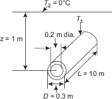
FIGURE Example 4.35 Isothermal cylinder of length L buried in a semi-infinite medium (L >> D and z > 1.5D)
Thermal resistances:
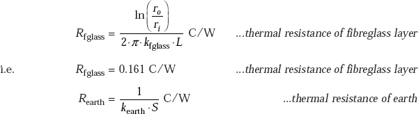
So, to calculate thermal resistance of earth, we need to calculate shape factor S, first.
Shape factor for this configuration is given in Fig. 4.21, as:
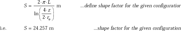
Therefore,
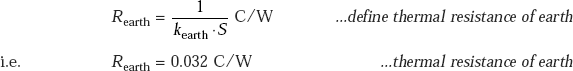
Heat transfer rate, Q:
To calculate temperature of outer surface of fibreglass insulation layer, T1:
Apply the Ohm’s law only to the fibreglass insulation layer: