Chapter 11
Boiling and Condensation
11.1 Introduction
In the previous two chapters, we studied heat transfer in forced and free convection, i.e. heat transfer with fluid motion, induced either by an external means or by density differences. In both the cases, fluid involved was homogeneous and in single phase. But, there are many important practical cases which involve heat transfer with a change of phase of the fluid, e.g. boiling where the liquid changes to vapour and condensation where the vapour condenses into a liquid. Boiling and condensation are classified under convection since there is motion of the fluid during heat transfer in these processes.
Some of the applications of boiling and condensation are:
- Evaporators and condensers of a vapour compression refrigerating system
- Boilers and condensers of a steam power plant
- Reboilers and condensers of distillation columns of cryogenic and petrochemical plants
- Cooling of nuclear reactors and rocket motors
- Process heating and cooling, etc.
Unique features of boiling and condensation are:
- heat transfer, practically at a constant temperature, because of change of phase
- latent heat and surface tension come into play in addition to buoyancy driven flow effects, resulting in larger heat transfer rates and heat transfer coefficients compared to the usual free or forced convection
- high heat transfer rates with small temperature difference.
11.2 Dimensionless Parameters in Boiling and Condensation
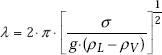
It is difficult to obtain governing equations for boiling and condensation by applying the usual conservation laws. However, dimensional analysis has been successfully applied with the use of Buckingham π theorem. Heat transfer coefficient in either boiling or condensation process may be reasonably assumed to depend on the temperature difference ΔT between the surface temperature Ts and the saturation temperature Tsat of the fluid, body force arising out of the density difference between the liquid and vapour phases {= g.(ρl – ρv)}, latent heat hfg, surface tension σ, a characteristic length L and the thermo-physical properties of the liquid or vapour; ρ, Cp, μ and k. Applying the Buckingham π theorem, it can be shown that the functional relationship between the various dimensionless groups is given by:
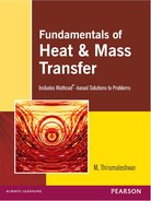
where, the dimensional groups are defined as follows:
The first term inside brackets in Eq. 11.1, i.e.
represents the effect of buoyancy induced fluid motion on heat transfer.
Jakob number (Ja) involves the ratio of maximum sensible energy absorbed to the latent heat absorbed. Generally, Ja has a small numerical value.
Bond number (Bo) is the ratio of gravitational body force to the surface tension force.
11.3 Boiling Heat Transfer
11.3.1 Boiling and Evaporation
’Boiling’ occurs at the solid-liquid interface when the solid surface is at a temperature Ts, sufficiently above the saturation temperature Tsat of the liquid at that pressure. In contrast, ‘evaporation’ occurs at the liquid-vapour interface when the vapour pressure above the liquid is less than the saturation pressure of the liquid at the given temperature. Unique feature of the boiling phenomenon is the production of vapour bubbles at the solid-liquid interface causing intense mixing.
11.3.2 Boiling Modes
Boiling is generally classified as ‘pool boiling’ and ‘flow boiling’.
In pool boiling, there is no bulk fluid flow, and any motion of the fluid is due to natural convection and the movement of bubbles under buoyancy effects. Heating of a liquid by immersing a heating element in it is an example of pool boiling. When boiling occurs while fluid is in motion under the influence of a pump, it is called flow boiling. These two modes of boiling are further classified as ‘sub-cooled boiling’ and ‘saturated boiling’. In sub-cooled boiling, main body of the liquid is at a temperature below the saturation temperature Tsat, while in saturated boiling, main body of the liquid is at a temperature equal to Tsat. During initial stages of boiling, we have the subcooled boiling where bubbles originate at the heating surface, move up due to buoyancy effects, and dissolve in the cooler liquid since the body of the liquid is at a temperature lower than Tsat. As the body of the liquid reaches the saturation temperature, bubbles start reaching up to the free surface of the liquid and we say that bulk or saturated boiling is set in motion.
Since boiling is a form of convection heat transfer, boiling heat flux is given by Newton’s law of cooling, i.e.
qboiling = h × (Ts − Tsat) = h × ΔTe W/m2 …(11.2)
where, ΔTe = (Ts – Tsat) = excess temperature.
11.3.3 Origin and Growth of Bubbles
Boiling is associated with bubble formation at the heating surface. Bubbles are believed to originate at the small cavities present on the heating surface by expansion of entrapped gas or vapour. These are known as ‘nucleation sites’. Then, the bubbles grow in size, detach themselves from the surface when a critical size is reached. Bubble growth and dynamics is closely related to the surface tension (σ) at the liquid - vapour interface, temperature excess and the pressure. Surface tension signifies the wetting capability of the liquid; lower the surface tension, higher the wetting capability.
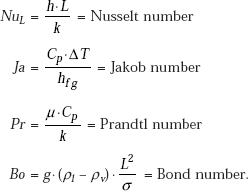
Wetting capacity of a liquid signifies the contact angle θ between the wall and the free surface. See Fig. 11.1.
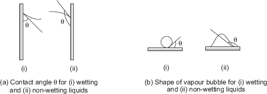
FIGURE 11.1 Contact angle and shape of vapour bubbles for wetting and non-wetting liquids
Larger the angle θ, poorer is the wetting capacity. A liquid is considered to wet a surface if θ < 90 deg. This is true for liquids like water (θ = 50 deg.), kerosene (θ = 26 deg.), ether (θ = 16 deg.) etc. If θ > 90 deg. liquid does not wet the surface, eg. mercury (θ = 137 deg.).
Based on theory of capillarity, following equation gives the separation diameter ‘d’ of a bubble in a quiet liquid:
where, θ is contact angle in deg., σ is surface tension in N/m, ρ is density of liquid or vapour in kg/m3.
For water boiling on a metal surface, Eq. 11.3 gets the following form:
At atmospheric pressure, for water, ρl = 957.9 kg/m3, ρv = 0.5978 kg/m3, and we get
d = 2.482 mm. Note that separation diameter diminishes with increasing pressure.
Intense mixing caused by the separation of the bubbles from the surface and their movement through the fluid results in high rate of heat transfer from the surface to the liquid. It is obvious that higher the number of nucleation sites where the bubbles originate and higher the frequency with which the bubbles detach from the surface, higher the heat transfer coefficient, h. Heat transfer coefficient is a function of excess temperature, ΔTe, as discussed below:
11.3.4 Boiling Regimes and Boiling Curve
Nukiyama performed his pioneering experiments on boiling heat transfer in 1934. He used nichrome and platinum wires which were electrically heated while immersed in liquids. In general, four different boiling regimes are observed depending upon the excess temperature (ΔTe) imposed, namely
- natural convection boiling (ΔTe upto about 5 deg.C)
- nucleate boiling (ΔTe from 5 deg to about 30 deg.C)
- transition boiling (ΔTe from 30 deg to about 120 deg.C), and
- film boiling (ΔTe beyond 120 deg.C).
Fig. 11.2 shows a typical boiling curve for water at one atmosphere pressure. General shape of the boiling curve is same for other fluids as well. In Fig. 11.2, boiling heat flux is plotted against the excess temperature. Also, shape of the boiling curve is independent of the geometry of the heating surface, but depends on the fluid pressure and the specific fluid-heating surface combination.
A brief explanation of the different boiling regimes is given below:
(i) Natural convection boiling This range is up to the point ‘A’ in Fig. 11.2. No bubbles are formed up to a small excess temperature of about 5 deg. and the liquid is superheated, rises to the free surface and evaporates from the surface. In this range, the free convection correlations derived in the previous chapter can be applied to make heat transfer calculations.
FIGURE 11.2 Typical boiling curve for water at one atmosphere pressure
(ii) Nucleate boiling Region between ‘A’ and ‘C’ is the nucleate boiling region. Starting from point ‘A’, as ΔTe increases, bubbles start forming at nucleation sites at an increasing rate. Nucleate boiling region may classified into two sub-regions:
- region A-B, where the isolated bubbles formed rise up, but do not reach the free surface and collapse in the body of the liquid; space vacated by the bubbles formed at the surface as they move up, is filled by fresh liquid, and the process is repeated. Movement of the bubbles through the body of the liquid causes agitation which is responsible for increasing heat transfer in nucleate boiling.
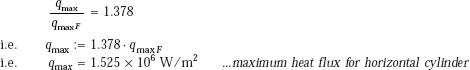
- region B-C, where the bubbles form at a faster rate at a largely increased number of nucleation sites and rise up in the liquid in almost continuous columns of vapour. These bubbles gush up in the liquid and reach the free surface and then collapse. Heat flux in this region is very large due to this reason. Note that after point B there is an inflection in the boiling curve; this is because of the fact that as excess temperature is increased, the heating surface gets almost covered with bubbles and the heat flux increases at a lower rate as ΔTe increases, and reaches a maximum at point C. Heat flux at point C is called ‘critical’ or ‘maximum’ or ‘burnout’ heat flux, qmax. For water, qmax > 1 MW/m2.
It should be clear that from heat transfer point of view, nulcleate boiling regime is the most desirable range to operate, since very high heat transfer rates are obtained with relatively small ΔTe .(under 30°C).
(iii) Transition boiling Region between ‘C’ and ‘D’ is the transition boiling region. In this range, as the excess temperature increases, the heat flux decreases; this is due to the fact that now a major portion of the heater surface is covered by the vapour film which has a smaller thermal conductivity as compared to that of the liquid, and, therefore, acts as an insulation. Between points C and D, nucleate and film boiling occur partially or alternately and is therefore called ‘unstable film boiling regime’. At point D, excess temperature is of the order of 120°C.
(iv) Film boiling This region is beyond the point D. As excess temperature is further increased, now a stable, vapour blanket completely covers the heater surface. So, at point D, the heat flux reaches a minimum and this point is known as ’Leidenfrost point’, (in honour of Leidenfrost, who explained in 1756 that the water drops dropped on a very hot surface ‘dance’ on a vapour film and boil away). Now, as the excess temperature is increased further, heat transfer by radiation effect also comes into picture in addition to conduction through the vapour film, and the heat flux increases as shown.
11.3.5 Burnout Phenomenon
In Fig. 11.2, a continuous boiling curve was shown. However, in practice, when Nukiyama conducted his experiments with an electrically heated nichrome wire immersed in a pool of water, he observed that when a little excess power was supplied to the nichrome wire after reaching point C, wire temperature suddenly increased uncontrollably to the melting point of the wire (i.e.1500 K) and burnout occurred. When the experiment was repeated with platinum wire (which has a higher melting point of 2045 K), it was possible to maintain heat flux higher than qmax without a burnout. Now, when the power was gradually reduced after qmin was reached at point D, there was a sudden drop in the excess temperature, landing into the nucleate boiling region. Note that the arm C-D of the boiling curve cannot be obtained in the power controlled mode of heating, unless the power applied is reduced suddenly when point C is reached. The phenomenon of ‘hysterisis effect’ explained above is shown in Fig. 11.3.

FIGURE 11.3 Actual boiling curve for water heated by a platinum wire
As we go on supplying electrical energy to the heater, point C (Fig. 11.2), i.e. the point of critical or maximum heat flux is reached; now, if we try to go past this point by increasing the heater power, the fluid is not able to accept this increased power as shown in Fig. 11.3, and as a result, the heater temperature increases. So, ΔTe increases, and the fluid can accept even lesser energy at this increased ΔT, and the heater temperature further increases, and so on. Thus, a steady state point E is reached in the boiling curve Fig. 11.2, which, unfortunately, corresponds to a very high surface temperature, that the heater may even melt or ‘burnout’. Hence, the name ‘burnout heat flux’ for the heat flux at point C.
Knowledge of ‘burnout flux’ is very important from practical point of view (in electrically heated surfaces and nuclear reactors), since any attempt to go past the point C of maximum heat flux will make the surface temperature to jump suddenly to point E, causing a burnout. So, the aim should be to operate at a point as near to the point C as possible, but never to go beyond it. In cryogenic applications, however, point E falls at temperatures much lower than the melting point of materials concerned, and film boiling can be adopted without any danger of a burnout.
11.3.6 Heat Transfer Correlations for Pool Boiling
There are different correlations for the different regimes of boiling discussed above. Most of these correlations are empirical, since, as already mentioned, phenomenon of boiling is not easily amenable to theoretical analysis.
Natural convection boiling regime (i.e. up to an excess temperature of about 5 deg.C). In this regime, the correlations already presented in the previous chapter on ‘Natural (or, Free) convection’ may be used.
Nucleate boiling regime (i.e. excess temperature varying from about 5 deg. up to about 30 deg.C). In this regime, heat transfer depends on the number of nucleation sites, rate of vapour bubble formation, etc. It is thought that much higher heat transfer rates obtained in this regime are due to the stirring and agitating effect caused by the bubbles on the surrounding liquid. Further, experiments show that nucleate boiling heat flux is not very much dependent on the geometry or orientation of the heater surface. Therefore, the correlation given below is valid for flat plates, cylinders and other geometries.
Correlation proposed by Rohsenow in 1952, is the most widely used one, for heat flux in the nucleate boiling regime:
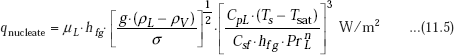
where,
qnucleate |
= nucleate boiling heat flux, W/m2 |
μL |
= viscosity of liquid, kg/(m.s) |
hfg |
= enthalpy of vaporisation, J/kg |
g |
= gravitational acceleration, m/s2 |
ρL |
= density of liquid, kg/m3 |
ρV |
= density of vapour, kg/m3 |
CpL |
= Specific heat of liquid, J/(kg.C) |
σ |
= surface tension of liquid-vapour interface, N/m |
Ts |
= surface temperature of heater, deg.C |
Tsat |
= saturation temperature of fluid, deg.C |
Csf |
= a constant depending upon the specific surface-fluid combination |
PrL |
= Prandtl number of liquid |
n |
= 1 for water, and 1.7 for all other liquids. |
Subscripts L and V refer to liquid and vapour, respectively.
Since water is one of the most common fluids used, it is useful to have its surface tension and the constant Csf for water-surface combination, readily available.
Surface tension and latent heat of water at a few temperatures are given in Table 11.1.
TABLE 11.1 σ and hfg for water
| Saturation temperature (Tsat), deg.C | Surface tension (σ), N/m | Latent heat (hfg), kJ/kg |
|---|---|---|
0 |
0.0755 |
2500.8 |
20 |
0.0729 |
2453.7 |
40 |
0.0695 |
2406.2 |
60 |
0.0661 |
2357.9 |
80 |
0.0627 |
2308.3 |
100 |
0.0589 |
2256.7 |
150 |
0.0487 |
2113.4 |
200 |
0.0378 |
1939.3 |
250 |
0.0261 |
1714.7 |
300 |
0.0143 |
1406.2 |
350 |
0.0036 |
916.1 |
374 |
0.0 |
0.0 |
A quick estimate of surface tension of water at a given temperature can be made using the following equation:
where, T is in deg.C
Experimentally determined values of constant Csf for a few liquid-surface combinations are given in Table 11.2:
Note that Rohsenow Eq. 11.5 is applicable for clean surfaces and for relatively smooth surfaces.
To calculate the heat flux in nucleate boiling, Collier recommends the following equation which is simpler to use as compared to Eq. 11.5:

where, ΔTe is the excess temperature in deg.C, P is the operating pressure in atm., Pcr is the critical pressure in atm.
Another correlation proposed by Mostinski to determine the heat transfer coefficient in nucleate boiling is:
TABLE 11.2 Csf for a few liquid-surface combinations
| Fluid and surface | Csf |
|---|---|
Water-copper: |
|
Scored surface |
0.0068 |
Polished surface |
0.0130 |
Water-stainless steel: |
|
Teflon coated surface |
0.0058 |
Ground and polished surface |
0.0068 |
Mechanically polished surface |
0.0130 |
Chemically etched surface |
0.0130 |
Water-brass |
0.0060 |
Water-nickel |
0.0060 |
Water-platinum |
0.0130 |
n-pentane-copper: |
|
Lapped surface |
0.0049 |
Polished surface |
0.0154 |
n-pentane-chromium |
0.0150 |
Ethyl alcohol-chromium |
0.0027 |
Benzene-chrommium |
0.101 |
where, P and Pcr are the operating and critical pressure (bar), respectively, ΔTe is the excess temperature in deg.C.
Once ‘h’ is known, heat flux is calculated as: q = h.ΔTe.
Another useful correlation for heat transfer coefficient in nucleate boiling is from Russian literature:
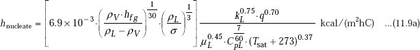
Note the units in the above equation: ρ in kg/m3, hfg in kcal/kg, σ in kg/m, k in kcal/(mhrC), μ in kgs/m2, Cp in kcal/(kgC) and subscripts L and V refer to liquid and vapour, respectively.
When all terms are expressed in S.I. Units, as in Eq. 11.5, above equation becomes:
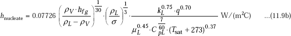
Advantage of Eq. 11.9b is that heat transfer coefficient is presented as a function of physical properties of the fluid only; therefore, it can be used to calculate ‘h’ for any fluid and at any pressure, if reliable data on physical properties are available.
Based on Eq. 11.9, following calculation formulas are recommended specifically for water in nucleate boiling, in the pressure range 0.2-100 ata:
hnucleate = 3.133 · q0.7 · P 0.15 W/(m2C) (for water …(11.10a))
and,
hnucleate = 45.054 · ΔT2.33 · P0.5 W/(m2C) (for water …(11.10b))
In the above equations q is the heat flux in W/m2, P is the pressure in bar, and ΔT is the excess temperature in deg.C.
Peak (or, maximum) heat flux in nucleate pool boiling:
During the design of heat transfer equipments (e.g. boiler tubes), it is extremely important to have an idea about the peak heat flux, so that steps can be taken to avoid a burnout.
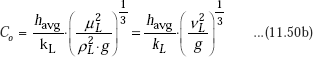
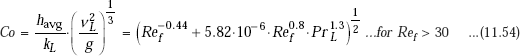
Leinhard and Dhir (1973) give the following correlation for peak heat flux in nucleate pool boiling:
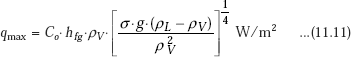
where, Co = 0.149 for a large horizontal surface
and, Co = 0.116 for a large horizontal cylinder.
Unlike the nucleate boiling flux, peak heat flux depends on heater geometry and orientation.
Eq. 11.11 indicates that water will have larger peak heat flux than any other common liquids, because of its large heat of vaporisation. Also, peak heat flux is a function of operating pressure, since the pressure affects the boiling point, which in turn, affects the heat of vaporisation and surface tension. According to experimental data, peak heat flux initially increases sharply as the pressure is increased, reaches a maximum, then decreases to zero at critical pressure. This trend is shown clearly for water, in Fig. 11.4.
In Fig. 11.4, on X-axis, we have the ratio of P/Pcr and on Y-axis is plotted the ratio (qpeak, p/qpeak, 1), where qpeak, p is the peak heat flux at the operating pressure P and qpeak, 1 is the peak heat flux at one atm. pressure. At the maximum point in the curve, we have:
P/Pcr = 0.35 and qpeak, p/qpeak, 1 = 3.2. Remembering that for water, Pcr = 225 ata, we see that qpeak = 4.652 × 10⁶ W/m2 must occur at P = 80 ata.
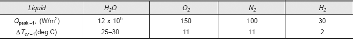
In addition to peak heat flux, the excess temperature at peak heat flux is also important to determine if the surface of the heater would reach the burnout point at a given peak heat flux. Experimental values of peak heat flux and the corresponding excess temperature are given in Table 11.3 for a few fluids at 1 atm. pressure:
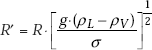
Another relation for peak heat flux on horizontal cylinders, which fits experimental data very well, is presented by Sun and Lienhard :
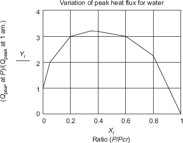
FIGURE 11.4 Variation of peak heat flux with pressure for water
TABLE 11.3 Peak heat flux and critical temperature for a few liquids at one atm. pressure
where, R’ is a dimensionless radius defined as:
and, qmax F is the peak heat flux on an infinite horizontal plate, given as:
Another useful correlation for peak heat flux in nucleate boiling is from Russian literature:
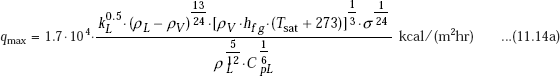
Note the units in the above equation ρ in kg/m3, hfg in kcal/kg, σ in kg/m, k in kcal/(m hr C), μ in kgs/m2, Cp in kcal/(kgC) and subscripts L and V refer to liquid and vapour, respectively.
When all terms are expressed in S.I. Units, as in Eq. 11.5, above equation becomes:
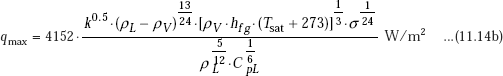
Advantage of Eq. 11.14b is that peak heat flux is presented as a function of physical properties of the fluid only; therefore, it can be used to calculate ‘qmax’ for any fluid and at any pressure, if reliable data on physical properties are available.
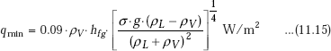
Minimum heat flux:
This occurs at point D in Fig. 11.2; minimum heat flux represents the lower limit of heat flux in film boiling. For a large, horizontal plate, Zuber derived the following relation (modified by Berenson in 1961) for minimum heat flux:
Film boiling:
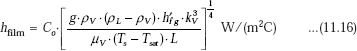
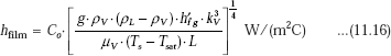
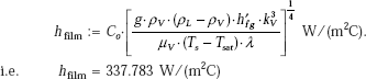
Heat transfer coefficient in stable film boiling regime on a horizontal cylinder or sphere is predicted by Bromley’s correlation:
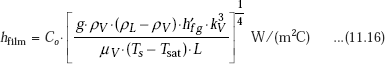
where,
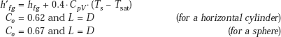
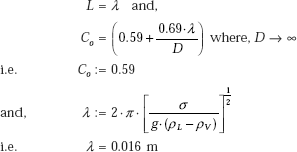
For a very large diameter tube (diameter D) or a horizontal surface, Eq. 11.16 is valid, with the following value for Co (Westwater and Breen, 1962):
and,
Note that for a horizontal surface, Co = 0.59, since D → ∞
Vapour properties in Eq. 11.16 are evaluated at the mean film temperature,
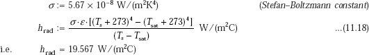
As stated earlier, during stable film boiling, at high temperatures (> 300°C), thermal radiation effects become significant and Bromley suggested using an overall heat transfer coefficient given by:
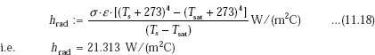
and, hrad is given by:
where, σ = 5.67 × 10⁻⁸ W/(m2K4) (Stefan–Boltzmann constant)
and, ε is the emissivity of the heated surface.
Also, remember that in Eq. 11.18, the temperatures Ts and Tsat must be in Kelvin.
Heat flux in stable film boiling is easily calculated, once the heat transfer coefficient is determined, i.e.
11.3.7 Simplified Correlations for Boiling with Water
Since water is one of the most commonly used fluids in practice, it is useful to have some simplified correlations for boiling water.
Jakob and Hawkins (1957) presented following simple relations for water boiling at atmospheric pressure on submerged surfaces:
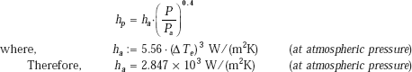
Heat transfer coefficients at pressures other than atmospheric may be calculated using the following empirical equation:
where, hp = heat transfer coefficient at any pressure p,
ha = heat transfer coefficient at pressure pa (= 1 atm.) from Table 11.4.
TABLE 11.4 Simplified relations for boiling heat transfer coefficient for water at one atm. pressure
| Type of surface | Range of validity (kW/m2) | h (W/m2K) |
|---|---|---|
Horizontal: |
qs < 15.8 15.8 < qs < 236 |
1040 × (ΔTe)1/3 5.56 × (ΔTe)3 |
Vertical: |
qs < 3.15 3.15 < qs < 63.1 |
539 × (ΔTe)1/7 7.95 × (ΔTe)3 |
Example 11.1. Water at a pressure of one atm. is boiled in a polished copper pan, 300 mm diameter. If the surface temperature of the pan is 110°C, (a) calculate the boiling heat flux and the heat transfer coefficient. What is the evaporation rate of water? (b) compare the nucleate boiling flux with the maximum heat flux (c) compare the values of heat transfer coefficient obtained from Rohsenow’s correlation with those obtained using Collier’s, Mostinski’s and Russian correlations.
Solution.
Data:
Ts := 110°C Tsat := 100°C d := 0.3 m Csf := 0.013 (from table 11.2)
Properties of water at Tsat = 100°C are:
ρL = 958.4 kg/m3 ρV = 0.5955 kg/m3 CPL = 4220 J/(kgK) μL = 279 × 10–6 kg/(ms) PrL = 1.75
hfg = 2257 × 103 J/kg σ = 58.9 × 10⁻³ N/m n = 1 (exponent n in eqn. 11.5) (exponent ‘n’ in eqn. 11.5)
g = 9.81 m/s2
Since ΔT is 10 deg.C, it is reasonable to assume that correlation for nucleate boiling regime is applicable. Then, we have, for heat flux:
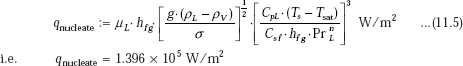
Heat transfer coefficient:
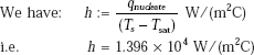
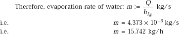
Evaporation rate:
(b) Maximum heat flux:
We have, from Eq. 11.11 for a horizontal surface:
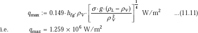
Thus, actual heat flux is much smaller than the critical (max) heat flux.
Let also check the actual heat flux using Collier’s correlation:
We have: |
Pcr := 225 atm |
(critical pressure for water) |
|
P := 1 atm |
(operating pressure) |
|
ΔTe := Ts − Tsat |
|
We have, from Collier’s correlation:
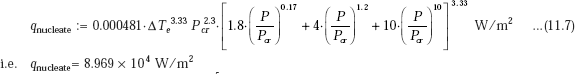
Compare this value with 1.396 × 10⁵, obtained using Rohsenow’s correlation.
Let us also check the actual heat flux using Mostinski’s correlation:
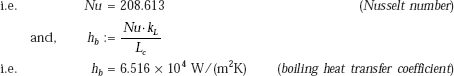
i.e. |
hnucleate = 8.739 × 10³ W/(m2C) |
and, |
qnucleate := hnucleate · ΔTe |
i.e. |
qnucleate = 8.739 × 10⁴ W/m2. |
Again, compare this value with 1.396 × 10⁵, obtained using Rohsenow’s correlation, and 8.969 × 10⁴, using Collier’s correlation.
Also, from Russian literature:
i.e. |
hnucleate = 9.632 × 10³ W/(m2C) |
and, |
qnucleate := h nucleate · ΔTe |
i.e. |
qnucleate = 9.632 × 10⁴ W/m2. |
Thus, it may be noted that these empirical relations can give values that differ from each other considerably. (c) comparing the values of h from different correlations:
|
h = 1.396 × 10⁴ W/(m2C) |
…Rohsenow’s correlation |
|
h = 8969 W/(m2C) |
…Collier’s correlation |
|
h = 8739 W/(m2C) |
…Mostinski’s correlation |
|
h = 9632 W/(m2C) |
…Russian correlation. |
Example 11.2. A nickel wire, 1 mm diameter and 300 mm long, is submerged in a water bath open to atmosphere. What is the value of current flowing through the wire that will cause burnout, if the applied voltage is 10 V?
Solution.
Data:
Tsat := 100°C R := 0.0005 m L := 0.3 m V := 10 V
Properties of water at Tsat = 100°C are:
ρL := 958.4 kg/m3 ρV := 0.5955 kg/m3 CpL := 4220 J/(kgK) μL := 279 × 10–6 kg/(ms) PrL := 1.75
hfg := 2257 × 103 J/kg σ := 58 × 10–3 N/m g := 9.81 m/s2
This is the case of a horizontal cylinder. So, let us use Eq. 11.12.
First, calculate the factor R’:
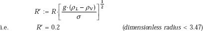
Therefore,
and, qmax F is the peak heat flux on an infinite horizontal plate, given as:
From Eq. 11.12a we get:
This is the value of burnout flux.
If V is the voltage, I the current through the wire, we have:
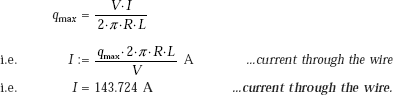
Example 11.3. A horizontal, metal-clad heating element, 10 mm diameter and of surface emissivity 0.85, is submerged in a water bath. Surface temperature of the heating element is 300°C. If the water is at atmospheric pressure, calculate the power dissipation per unit length of the heater.
Solution.
Data:
Tsat := 100°C D := 0.01 m L := 1 m Ts := 300°C ε := 0.85 ρL := 958.4 kg/m3
hfg := 2257 × 103 J/kg g := 9.81 m/s2 σ := 5.67 × 10⁻⁸ W/(m2K4)
Since the excess temperature is (300 – 100) = 200°C, it is film boiling region. We need properties of vapour at the mean film temperature of (300 + 100)/2 = 200°C.
Properies of vapour at 200°C:
kV := 0.0375 W/(mK) ρV := 7.85 kg/m3 μV := 15.7 × 10⁻⁶ kg/(ms) CpV := 2910 J/(kgK)
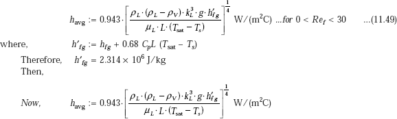
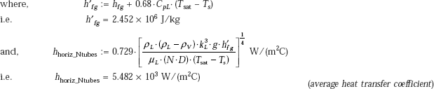
h′fg := hfg + 0.4 CpV.(Ts - Tsat) i.e. h′fg := 2.49 × 10⁶ J/kg
Then, for a horizontal cylinder, we have:
with Co = 0.62 and L = D…for a horizontal cylinder
Radiative heat transfer coefficient is given by:
Therefore, the ‘total’ heat transfer coefficient is given by:
h : = hfilm + 0.75 · hrad …(11.17)
i.e. h = 477.145 W/(m2C)
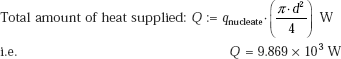
Therefore, power dissipation per unit length of heater:
Q : = h · (π · D · L) · (Ts − Tsat) W/m
i.e. Q = 2.998 × 10³ W/m.
Example 11.4. A large, horizontal plate is kept immersed in a water bath boiling at 1 atm, 100°C. Surface temperature of the plate is 260°C. Calculate the heat transfer coefficient and the heat flux. Assume the emissivity of the surface as 0.9.
Solution.
Data:
Tsat := 100°C Ts := 260°C ε := 0.9 ρL := 958.4 kg/m3 hfg := 2257 × 103 J/kg
g := 9.81 m/s2 σ := 58.9 × 10⁻³ N/m
Since the excess temperature is (260-100) = 160°C, it is film boiling region. We need properties of vapour at the mean film temperature of (260 + 100)/2 = 180°C.
Properties of vapour at 180°C:
kV := 0.03268 W/(mK) ρV := 5.16 kg/m3 μV := 15.1 × 10⁻⁶ kg/(ms) CpV := 2709 J/(kgK)
h′fg := hfg + 0.4 · CpV · (Ts – Tsat) i.e. h’fg := 2.43 × 10⁶ J/kg
Then, we apply Eq. 11.16:
where, for a horizontal surface, we have:
Then, film boiling heat transfer coefficient:
And, radiative heat transfer coefficient:
Note: Use absolute temperatures in Eq. 11.18 for radiative heat transfer.
Therefore, the ‘total’ heat transfer coefficient is given by:
h : = hfilm + 0.75 · hrad …(11.17)
i.e. h = 352.458 W/(m2C)
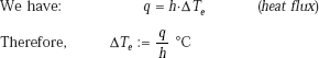
and, the heat flux:
q := h × (Ts − Tsat) W/m2
i.e. q = 5.639 × 10⁴ W/m2.
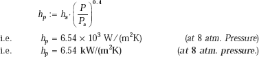
Example 11.5. Water is boiling at 8 atm. on the surface of a horizontal tube, whose wall temperature is maintained at 8°C above the boiling point of water. Calculate the nucleate boiling heat transfer coefficient
(b) What is the change in the value of heat transfer coefficient when (i) temperature difference is increased to 16°C at the pressure of 8 atm., and (ii) pressure is raised to 16 atm. with ΔTe = 8°C.
Solution.
Data:
ΔTe := 8°C Pa := 1 atm P := 8 atm
Now, we use the following relation (assuming q > 15.8 kW/m2), from Table 11.4:
and,
(i) Now, when the ΔT is increased to 16°C, with the pressure remaining at 8 atm.:
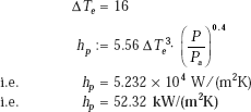
i.e. heat transfer coefficient increases by about 8 times as compared to the earlier value when ΔT was 8°C.
(ii) When the pressure is increased to 16 atm., with the ΔT remaining at 8°C.:
Again, we have:
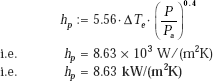
i.e. heat transfer coefficient increases by about 32% as compared to the original value at a pressure of 8 atm.
11.3.8 Flow Boiling
Flow boiling or boiling in forced convection, is important in the design of boiling nuclear reactors, in spacecrafts and space power systems.
In flow boiling, a fluid is forced to move over a heated surface while the phase change occurs. Therefore, combined effects of natural/forced convection and pool boiling come into play.
Flow boiling is classified as:
- External flow boiling, and
- Internal flow boiling.
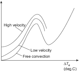
FIGURE 11.5 Effect of flow velocity in external flow boiling
(i) External flow boiling In external flow boiling, flow occurs over the surface of a plate or cylinder; there are the flow regimes similar to that in pool boiling, but due to the effect of flow velocity, both the nucleate boiling heat flux and the critical heat flux get enhanced. See Fig. 11.5. For water in external flow boiling, critical heat flux value as high as 35 MW/m2 has been obtained (as compared to the value of 1.3 MW/m2 in pool boiling at one atm.).
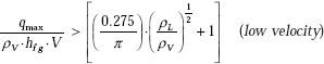
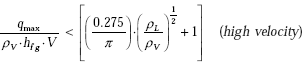
For cross flow over a cylinder of diameter D, Lienhard and Eichhorn have given following correlations, depending upon whether the fluid velocity is ‘low’ or ‘high’.
Criterion to determine if the velocity is low or high is:
and,
Correlation for low velocity:
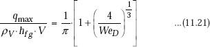
Correlation for high velocity:
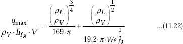
Here, V is the fluid velocity and WeD is the Weber number, defined as the ratio of inertia forces to surface tension forces, i.e.
(ii) Internal flow boiling Internal forced convection boiling refers to flow inside a tube. This is more complicated since, now, there is no free surface for the vapour to escape and results in two phase flow inside the tube. There are different flow regimes occurring inside the tube depending upon the ‘quality’ of the fluid. (‘Quality’ is defined as the ratio of mass of vapour to the total mass of fluid at a given location). This is illustrated in Fig. 11.6, which also shows a qualitative graph of variation of heat transfer coefficient with local quality.
Consider a fluid, at a temperature below its boiling point, entering a vertical, heated tube. Progressive vaporisation occurs along the length of the tube and the ‘quality’ increases. Up to a short distance from the inlet, heat transfer coefficient for the single phase fluid may be predicted using the Dittus-Boelter equation.
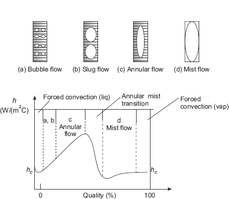
FIGURE 11.6 Flow regimes and heat transfer coefficient in forced convection flow in a vertical tube
Bubble-flow regime Soon, the bulk temperature reaches the saturation point, and bubbles are formed at the nucleation sites on the wall and are carried into the main stream, as in nucleate boiling. This is known as the ‘bubble flow regime’ (see Fig. 11.6 (a)) and the heat transfer coefficient increases. Heat transfer coefficient in this range can be predicted by superimposing the liquid-forced convection and nucleate pool boiling equations.
Slug-flow regime Further along the distance, vapour fraction increases and individual bubbles agglomerate and slugs of vapour are formed. This regime is known as ‘slug flow regime’. See Fig. 11.6 (b). Fluid velocity increases and since the slugs of vapour are compressible, flow oscillations may occur. Mass fraction of vapour in this regime is around 1 %, but volume fraction of vapour may be even up to 50 %. In this regime also, heat transfer coefficient may be calculated by superimposing the liquid-forced convection and nucleate pool boiling equations. Heat transfer coefficient increases because of increased velocity.
Annular-flow regime As the fluid progresses further up the tube, quality increases due to further addition of heat and vapour forms the core and a film of liquid flows on the inner wall surface. Vapour core travels at a higher velocity than the liquid and vapours are formed primarily at the liquid-vapour interface and not at the wall surface. Quality in this flow regime may be up to 25 %. See Fig. 11.6 (c).
Transition-flow regime Now, as the quality increases, there is a sudden drop in the value of heat transfer coefficient. Heat flux at this point is known as ‘critical heat flux’. This is the point of dryout. This sudden drop happens since the liquid film at the wall is now replaced by a vapour film, which has a poor thermal conductivity. There may be sharp increase in the wall temperature and even burnout may occur.
Mist-flow regime Now, the tube is fully occupied by the vapour, which may contain droplets of liquid. This is known as mist-flow regime. See Fig. 11.6 (d). Heat transfer is from the wall to the vapour directly, and then from the vapour, heat is transferred to the droplets of liquid contained in the vapour.
From the annular-flow regime onwards, prediction of heat transfer coefficient is a little difficult and uncertain due to problems of two phase flow.
Correlations to find out heat transfer coefficient in nucleate flow boiling as well as in two-phase flow boiling are presented below:
Correlations for nucleate flow boiling:
Rosenhow and Griffith (1955) have suggested that total heat flux be calculated by adding the nucleate pool boiling flux (from Eq. 11.5) and the forced convection effect (from Dittus-Boelter equation with the coefficient 0.023 replaced by 0.019),
i.e.
For forced convection flow inside vertical tubes, following correlation is recommended:
where, ΔTe = Ts – Tsat , and p = pressure in mega pascals.
Above equation is valid for the pressure range of 5 to 170 bar.
For horizontal tubes, McAdams et.al. suggest following relation for low pressure boiling water:
q = 2.253 · (Δ Te)3.96 W/m2 …for 0.2 < P < 0.7 MPa …(11.25a)
For higher pressures, Levy recommends:
Here, the pressure P is in mega-Pascals.
Correlations for two-phase, flow boiling:
Beyond the saturated nucleate boiling, there is annular-flow region, and Chen’s correlation (1966) has been widely used for two-phase heat transfer calculations.
Here,
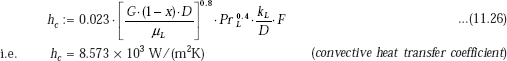
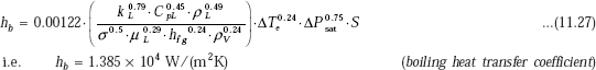
where, hc is the contribution due to annular region and hb is the contribution due to nucleate boiling region. We have:
and,
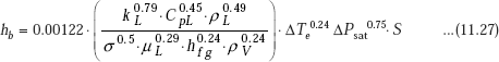
ΔPsat = change in vapour pressure corresponding to a temperature change of ΔTe.
‘v’ is the specific volume.
S.I. Units are used throughout.
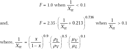
Parameter F is calculated from:
Parameter S is given by:
S = (1 + 0.12 · ReTP1.14)−1 for ReTP < 32.5
S = (1 + 0.42 · ReTP0.78)−1 for 32.5 < ReTP < 70
S = 0.1 for ReTP > 70
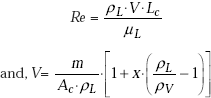
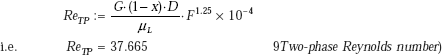
where, Reynolds number ReTP is defined as:
Chen’s correlation has been tested for several systems (including water) for pressures ranging from 0.5 to 35 atm and quality ‘x’ ranging from 1 to 71%.
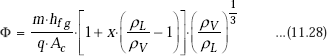
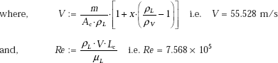
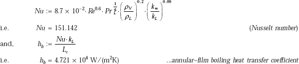
More recent correlation For flow boiling, recent correlation is due to Klimenko (1988). This is for a liquid boiling at a pressure P, in a pipe with a wall thermal conductivity of kw and cross-sectional area Ac. This correlation is valid for both nucleate boiling and annular film boiling up to dry out.
First, we have to determine whether it is nucleate flow boiling regime or annular film boiling regime. This is done by evaluating parameter ϕ:
Quality ‘x’ is defined as:
where, mV is the mass of vapour and mL is the mass of liquid, and m = (mV + mL)
Nucleate flow boiling (ϕ < 1.6 × 10⁴):
where,
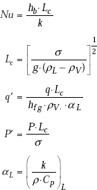
Annular film boiling (ϕ > 1.6 × 10⁴):
where,
All properties are evaluated at temperature Tsat.
The actual, effective heat transfer coefficient due to boiling and single phase forced convection is obtained
Example 11.6. Water at 8 atm. flows inside a vertical tube of 2.5 cm diameter under flow boiling conditions. Tube wall temperature is maintained at 8°C above the saturation temperature. Determine the heat transfer for one metre length of tube.
Solution.
Data:
D := 0.025 m L := 1 m ΔTe := 8°C P := 8 atm i.e. P := 8.0 × 0.10132 MPa i.e. P := 0.811 MPa
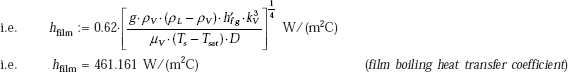
We apply Eq. 11.25
where, P is in mega Pascals
Therefore, h = 2.193 × 10³ W/(m2K)
Then, heat transfer for 1 m length of tube:
Q := h · (π · D · L) · ΔTe W/m
i.e. Q : = 1.378 × 10³ W/m.
Example 11.7. A 50 mm diameter vertical evaporator tube (kw = 20 W/(mK)) carries 1 kg/s of steam at 14.55 bar at a quality x = 0.2. The tube is subjected to a uniform heat flux of 106 W/m2. Identify the regime of flow boiling and calculate the convective heat transfer coefficient and surface temperature of the tube.
(b) when the quality reaches 0.8, what is the boiling regime and how much is the boiling heat transfer coefficient?
Solution.
Data:
D := 0.05 m P := 14.55 × 10⁵ N/m2 Tsat := 470 K(at 14.55 bar) hfg := 1951 × 103 J/kg (at 14.55 bar)
m := 1 kg/s x := 0.2 kw := 20 W/(mK) ρL := 868.056 kg/m3 ρV := 7.353 kg/m3 kL := 0.667 W/(mK)
CpL := 4480 J/(kgK) μL := 136 × 10–6 N.s/m2 PrL := 0.92 σ := 0.0385 N/m (surface tension)
q := 106 W/m2 g := 9.81 m/s2
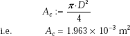
Cross-sectional area of tube:
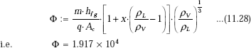
First, find out the parameter Φ to determine if the flow boiling regime is nucleate or annular-film:
We have:
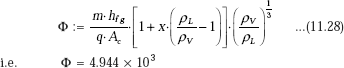
Since Φ < 1.6 × 10⁴, it is nucleate flow boiling regime.
Heat transfer coefficient:
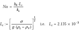
We use Klimenko’s correlation to determine the boiling heat transfer coefficient hb.
From Eq. 11.30:
where,
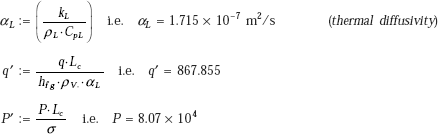
Therefore,
Single-phase forced convection heat transfer coefficient hc:
We use Dittus-Boelter equation, namely,
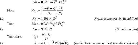
Therefore, total or effective heat transfer coefficient:
Total or effective heat transfer coefficient is given by Eq. 11.32:
Tube surface temperature:
i.e. |
ΔTe = 15.345°C |
|
and, |
Ts := Tsat + ΔTe |
|
i.e. |
Ts = 485.345 K |
|
i.e. |
Ts = 212.345°C |
(tube surface temperature.) |
(b) When quality, x = 0.8:
We have:
Since Φ > 1.6 × 10⁴, it is annular-film flow boiling regime.
In this regime, Klimenko’s correlation for boiling heat transfer coefficient is:
Therefore,
Compare this value with hb = 6.516 × 10⁴, obtained earlier for nucleate flow boiling. It is as it should be, since in annular film flow boiling, the heat transfer coefficient is less than that in the nucleate flow boiling.
Example 11.8. In Example 11.7, if the tube surface is maintained at a constant temperature of 227°C, calculate the total heat transfer coefficient and surface heat flux at the point where the quality is 0.2. Rest of the data are the same as in Example 11.7.
Solution.
Data:
D := 0.05 m P := 14.55 · 105 N/m2 Tsat := 470 K (at 14.55 bar) hfg := 1951 × 103 J/kg Ts := 500 K
∴ ΔTe := Ts - Tsat Ps := 26.4 bar, corresponding to 500 K i.e. ΔPsat := (26.4 – 14.55) × 105 N/m2 m := 1 kg/s
x := 0.2 (quality) ρL := 868.056 kg/m3 ρV := 7.353 kg/m3 kL := 0.667 W/(mK) CpL := 4480 J/(kgK)
μL := 136 × 10–6 Ns/m2 μV := 15.54 × 10⁻⁶ Ns/m2 PrL := 0.92 σ := 0.0385 N/m g := 9.81 m/s2
Cross-sectional area of tube:
Now, let us use Chen’s correlation.
We have:
where, hc is the contribution of single-phase convection and hb is the contribution of boiling region.
and,
First, let us calculate 1/Xtt, so that factor F can be calculated:
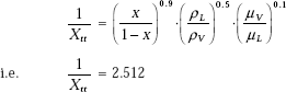
This is greater than 0.1. Therefore,
i.e. F = 2.091
Also, G, the mass velocity is:
Then, we have:
and, to calculate hb, we need to calculate the factor S, after finding out ReTP,:
Then, we have:
Therefore,
Then, total heat transfer coefficient h:
h := hc + hb
i.e. h = 2.243 × 10⁴ W/(m2K) (total heat transfer coefficient)
And, surface heat flux at that point where x = 0.2:
q := h · ΔTe
q = 6.728 × 10⁵ W/m2 (local heat flux.)
11.4 Condensation Heat Transfer
11.4.1 Introduction
Condensation heat transfer has important practical applications, e.g. in thermal power plants, low pressure exhaust steam from the steam turbine is condensed on the outside of water cooled tubes of a condenser; in vapour compression refrigeration and air-conditioning systems, the refrigerant is condensed inside tubes of the condenser, in the condenser-reboiler of cryogenic distillation columns, etc.
Whenever a saturated vapour at a temperature Tsat is brought in contact with a surface maintained at temperature Ts such that Ts is less than Tsat, vapours condense on the surface. Thus, in a way, condensation is the ‘reverse’ of boiling process. While condensing, naturally, the vapours will release the latent heat of vaporisation.
The vapours may condense on the surface in one of the two modes: ‘film-wise condensation’ or ‘drop-wise condensation’.
In film-wise condensation, say, on a vertical surface, vapours condense on the surface and drip down forming a continuous liquid film on the surface. Thickness of the condensate film increases as it travels down towards the lower (or trailing) end of the plate. During the condensation process, latent heat of vaporisation is released by the vapours. For further condensation to occur, the released latent heat has to be conducted through this liquid film to the cooled surface at temperature Ts. However, the liquid film offers resistance to the flow of heat and this resistance increases as the thickness of the film grows. Film-wise condensation occurs on surfaces which tend to get ‘wetted’.
In drop-wise condensation, the vapours condense on the surface on drops, which drip down the surface. A continuous film of liquid is not formed on the surface. Thus, more of the base area at temperature Ts is always exposed to the vapours. Therefore, heat transfer rate is higher (up to ten times) in drop-wise condensation as compared to the value in film-wise condensation. Generally, drop-wise condensation occurs on smooth surfaces which do not get ‘wetted’.
While drop-wise condensation would appear to be the preferred mode, in practice, it is difficult to maintain this mode of condensation since, with time, all surfaces tend to get wetted.
Attempts to achieve drop-wise condensation have been made either by coating the surface with some suitable material or by adding some additives to the vapours; but, commercially, these techniques have not yet become viable.
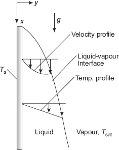
FIGURE 11.7 Film condensation on a vertical plate
11.4.2 Film Condensation and Flow Regimes
Consider film condensation of a vapour at saturation temperature Tsat on the surface of a cooled vertical plate, maintained at a temperature Ts (< Tsat.). See Fig. 11.7.
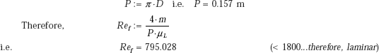
Vapour condenses on the top of the plate and flows down as a film. Thickness of the film (δ) is zero at the top of the plate (i.e. at x = 0 in the coordinate system shown) and increases as we travel down the plate (i.e. as x increases) due to additional condensation of vapour. Initially, the liquid film flow is laminar; after some distance it will become wavy and later, it may even turn turbulent. These different flow regimes are identified according to a ‘film Reynolds number’, defined as follows:
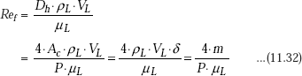
where,
Dh = 4Ac/P = 4.δ = hydraulic diameter of condensate flow, m
P = wetted perimeter of condensate, m
Ac = P.δ = area of cross section of flow at the lowest part of flow, m2
ρL = density of liquid, kg/m3
μL = viscosity of liquid, kg/ms
VL = average velocity of condensate at the lowest part of flow, m/s
ρLAcVL = m = mass flow rate of condensate at the lowest part of flow, kg/s.
For the common geometries of a vertical plate, vertical cylinder and a horizontal cylinder, hydraulic diameter Dh is equal to 4 times the thickness of the condensate, δ, at the location where the hydraulic diameter is to be evaluated; this is clearly shown as follows:
For a vertical plate Let B be the breadth of the plate, perpendicular to paper. At any section along the vertical height, let the thickness of the liquid film be δ. Then,
|
Ac |
= B.δ = area of cross section |
|
P |
= B = wetted perimeter, and |
|
Dh |
= 4.Ac/P = 4.δ. |
For a vertical cylinder Let D be the diameter of the cylinder. At any section along the vertical height, let the thickness of the liquid film be δ. Then,
|
Ac |
= π.D.δ = area of cross section |
|
P |
= π.D = wetted perimeter, and |
|
Dh |
= 4.Ac/P = 4.δ. |
For a horizontal cylinder Let D be the diameter of the cylinder, and L the length. Along the length of the cylinder, let the thickness of the liquid film be δ. Then,
|
Ac |
=2.L.δ = area of cross section |
|
P |
= 2.L = wetted perimeter, and |
|
Dh |
= 4.Ac/P = 4.δ. |
Again, considering Eq. 11.32, for a vertical plate, wetted perimeter, P = B, the breadth; therefore, (m/P) is the mass flow rate per unit breadth. If we denote (m/P) by m’, we can write for the vertical plate:
Another point to be noted is regarding the latent heat of vaporisatiion (hfg) released during condensation: Vapour at a temperature of Tsat comes in contact with the plate at a temperature of Ts (< Tsat) and condenses. However, the condensed liquid is, invariably, further sub-cooled to a temperature somewhere in between Ts and Tsat, thus releasing some more heat. Rohsenow (1956) suggested that this subcooling of the liquid can be taken into account by replacing hfg by a ’modified latent heat of vaporisation’, h’fg, defined as:
where, CpL is the specific heat of liquid at the average film temperature.
Similarly, if a superheated vapour at a temperature, Tv, enters a condenser and condenses, the superheated vapour has to be cooled to Tsat first, and then condensed at Tsat, and then sub-cooled to some temperature between Ts and Tsat. Then, modified latent heat of vaporisation is:
where, CpV is the specific heat of vapour at the average temperature of (TV + Tsat)/2.
Then, rate of heat transfer in condensation becomes:
where, A is the surface area on which condensation occurs.
Then, from Eq. 11.35 and 11.32, we can write:
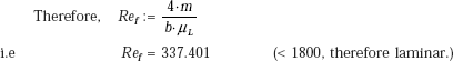
When either Qconden or h is known, it is convenient to use Eq. 11.36 to determine Ref.
Now, different flow regimes are identified according to the value of Ref as follows:
Ref ≤ 30 |
(Liquid film is smooth and wave-free, i.e. fully laminar.) |
450 < Ref < 1800 |
(Liquid film has ripples or waves and the flow is wavy—laminar.) |
Ref > 1800 |
(Liquid film is fully turbulent.) |
Heat transfer correlations vary depending upon the flow regime.
11.4.3 Nusselt’s Theory for Laminar Film Condensation on Vertical Plates
Nusselt developed his theory for laminar film condensation on vertical plates analytically in 1916.
Consider a vertical plate maintained at a temperature Ts and exposed to a saturated vapour at a temperature of Tsat. (Ts < Tsat). See Fig. 11.8. Let the height of the plate be L and the breadth, ’b’. Coordinate system is chosen such that x-coordinate is to the downward direction, i.e. in the direction of flow of condensate and y-coordinate is towards the right, as shown. Condensation occurs on the plate and the condensate moves down from top to bottom. Thickness of condensate is zero at the top (i.e. at x = 0) and increases in the flow direction, due to additional condensation of vapour. Since the liquid film offers resistance to the flow of heat from the vapour to the cold surface, this also means that resistance to heat transfer is minimum at the top of the plate and the resistance increases as one moves down in the flow direction.
Nusselt made the following simplifying assumptions in his analysis:
- Flow of liquid film is laminar
- Inertia force in the film is negligible (i.e. negligible acceleration of the liquid in the film) compared to viscosity and weight
- Heat flow is mainly by conduction through the liquid film; convection in liquid as well as in vapour is neglected.
- Temperature is Ts at the liquid-plate interface and Tsat at the liquid-vapour interface and the temperature gradient between them is linear
- Velocity of vapour is low, i.e. there is no viscous shear force at the liquid-vapour interface
- Properties of the liquid are constant.
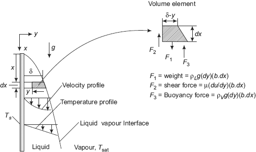
FIGURE 11.8 Film condensation on a vertical plate—Nusselt’s analysis
Velocity profile:
Considering a volume element as shown, apply Newton’s second law to get the velocity profile:
since the acceleration of the liquid film is negligible… by assumption.
So, making the force balance:
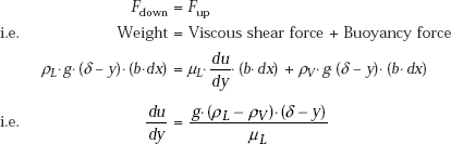
Integrating from y = 0 (i.e. the plate surface) to y = y, and remembering that at y = 0, u = 0, and at y = y, u = u(y), we get:
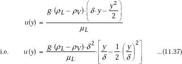
Eqn. 11.37 is the desired equation for velocity profile.
And, the mean flow velocity of the liquid at a section is given by:
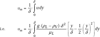
Mass flow rate:
Mass flow rate of condensate through any x-position is given by:
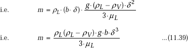
Note that mass flow rate is a function of position (x), since the film thickness δ is function of x.
As we proceed from position x to (x + dx), film thickness increases from δ to (δ + dδ), and there is additional mass ’dm’ condensed. This additional mass ’dm’ condensed between x and (x + dx) is obtained by differentiating Eq. 11.39 w.r.t. x (or δ):
Heat flow rate:
While condensing ‘dm’ amount of liquid, certain amount of latent heat of vaporisation is released; this is equal to:
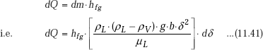
But, as per the assumption, heat flow through the liquid film is by pure conduction, with linear temperature gradient. Therefore, we can write:
From Eqs. 11.41 and 11.42:
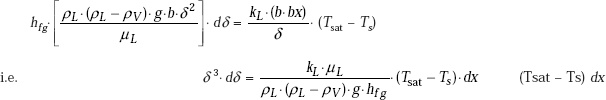
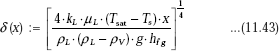
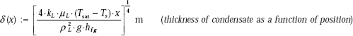
Integrating the above equation with the boundary condition that δ = 0 at x = 0, we get:
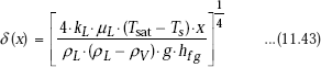
Eq. 11.43 gives the liquid film thickness as a function of position x. Note that the film thickness increases as the fourth root of the distance along the flow direction. Increase is rapid at the top end of the vertical plate and slows down later.
Heat transfer coefficient:
For the heat flow through the liquid film, we have:
Also, by Newton’s law of cooling:
where, hx is the local heat transfer coefficient
From the above two relations, we get:
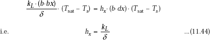
Note that at any position along the height, heat transfer coefficient is directly proportional to the thermal conductivity kL of the condensate and inversely proportional to the thickness of the film.
Substituting the value of δ from Eq. 11.43 in Eq. 11.44:
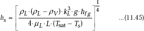
At x = L, i.e. at the lower end of the plate, local heat transfer coefficient is:
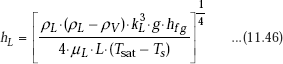
Obviously, rate of condensation heat transfer is higher at the upper end as compared to that at the lower end.
Average value of heat transfer coefficient over the entire height of the plate is of interest to calculate the total heat transfer rate. This is obtained by integrating Eq. 11.45 over the height L:
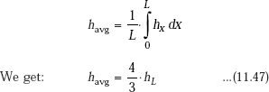
In the above, hL is the local heat transfer coefficient at x = L, i.e. at the lower end of the plate. Substituting for hL from Eq. 11.46, we get:
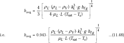
Eq. 11.48 is Nusselt’s equation for average heat transfer coefficient for condensation on a vertical plate.
It is observed that in practice, experimental value of average heat transfer coefficient is about 20% higher than that given by Nusselt’s Eq. 11.48. So, McAdams suggested to use a coefficient of 1.13 instead of 0.943 in Eq. 11.48.
Nusselts equation underpredicts the value of h, basically because:
- it does not take into account non-linear temperature profile in the liquid film, and
- it does not take into account the sub-cooling of the liquid film.
These effects can be accounted for by replacing hfg in Eq. 11.48 by h’fg given by Eq. 11.33.
Then, we have, for average heat transfer coefficient for laminar film condensation on a vertical plate:
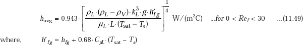
In the above equation all the liquid properties should be evaluated at the film temperature,
It is desirable to get relations for heat transfer coefficient in terms of the film Reynolds number. Now, let us define a dimensionless number called ’Condensation number’, (Co) [or, ‘modified Nusselt number’] as follows:
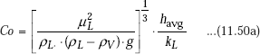
Since, ρL >> ρV, condensation number can be simplified as:
Then, Rohsenow (1985) has shown that above derived relation for heat transfer coefficient for condensation on a vertical plate for the laminar regimes of condensate flow, can be re-cast as follows:
(a) Laminar flow, (Ref ≤ 30):
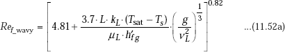
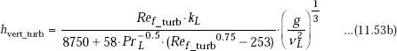
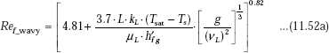
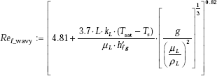
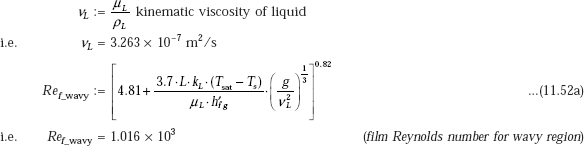
(b) In the laminar-wavy region, (30 < Ref < 1800):
Kutatelazde recommends following correlation:
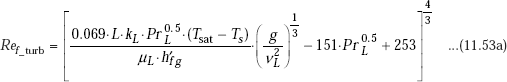
(c) For turbulent region, (Ref > 1800):
Labuntsov recommends following correlation for turbulent film condensation:
Eqs. 11.51, 11.52 and 11.53 are depicted graphically in Fig. 11.9 below:
From Eq. 11.53, it may be observed that in the turbulent film condensation region, the condensation number depends on liquid Prandtl number, PrL, too, in addition to the film Reynolds number, Ref. This Prandtl number dependence of Co in turbulent film region is clearly shown in Fig. 11.9 for PrL = 1, 3, 5 and 10.
Above correlations for condensation on a vertical plate are applicable to condensation inside or outside vertical tubes also, if the tube diameter is not too small.
Calculation formulas for all the three regions of film condensation on a vertical plate (or cylinder) are given below:
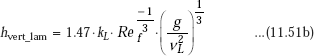
Calculation formulas for laminar region, for vertcal plate are:
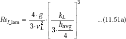
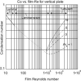
FIGURE 11.9 Condensation number vs. film Reynolds number for a vertical plate
where, havg is from Eq. (11.49)
and,
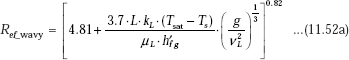
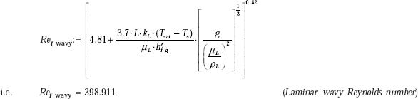
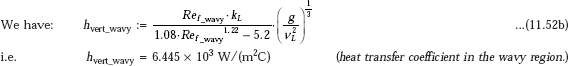
Calculation formulas for laminar-wavy region, for vertcal plate are:
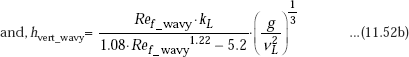
Calculation formulas for turbulent film region, for vertcal plate are:
and,
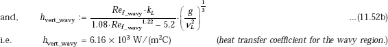
Chen et.al. (1987) have suggested the following universal correlation for both wavy and turbulent regions (instead of Eqs. 11.52 and 11.53) for condensation on a vertical plate:
11.4.4 Film Condensation on Inclined Plates, Vertical Tubes, Horizontal Tubes and Spheres, and Horizontal Tube Banks
Inclined plates:
Eq. 11.49 for laminar condensation on vertical plates can also be used for inclined plates. If the plate is inclined at an angle of θ to the vertical, (θ< 60 deg.), replacing g by g.cos(q) in Eq. 11.49 gives satisfactory results for laminar condensation on the upper surface of the inclined plate, i.e.
We can also write:
Vertical tubes:
Eq. 11.49 for laminar condensation on vertical plates can also be used to determine heat transfer coefficient for laminar condensation on the outer or inner surface of a vertical tube, if the tube diameter is large compared to the thickness of the liquid film, i.e.
if D>> δ
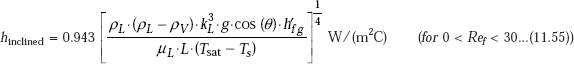
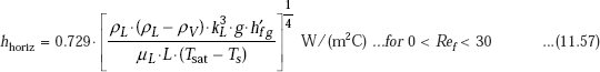
Horizontal tubes and spheres:
Horizontal tube-laminar film condensation:
For laminar film condensation on horizontal tubes and spheres, Nusselt type of analysis gives relations similar to Eq. 11.49, except that L is replaced by diameter D and the value of the numerical constant is different. We get:
Horizontal tube-forced convection condensation:
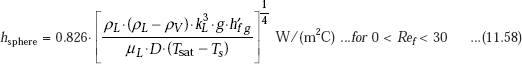
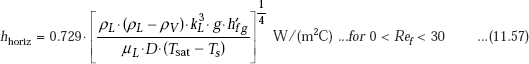
Eq. 11.57 is for the case of a quiescent vapour condensing on a horizonal tube. However, for condensers used in practice, a vapour may be forced through a condenser while being condensed. For the case of a cylinder of diameter D exposed to cross flow of a vapour with a free stream velocity of U, following correlation due to Shekriladze and Gomelauri (1966), may be applied:
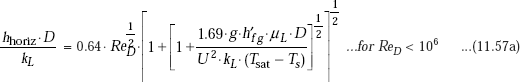
where, ![]()
Sphere-laminar film condensation:
It is interesting to compare the laminar condensation on vertical and horizontal tubes. From Eqs. 11.49 and 11.57, we can write:
For hvert to be equal to hhoriz, we should have:
L = (1.294)4 ·D
i.e. L = 2.8 · D
i.e. for L > 2.8.D, heat transfer coefficient will be higher for a horizontal tube. It is a fact that most of the tubes used in practice have lengths such that L > 2.8.D. Therefore, tubes used in a steam condenser are generally arranged in a horizontal orientation.
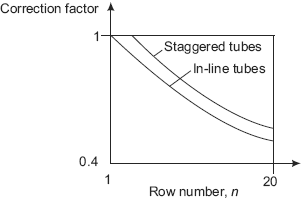
FIGURE 11.10 Correction factor for heat transfer coefficient in different rows of a condenser
Horizontal tube banks:
More than a single horizontal tube, an array of horizontal tubes condensing a vapour on their outer surfaces is of practical interest. In a steam condenser, generally such an array of tubes is used to condense low pressure steam exiting from the steam turbine. These tubes are cooled by circulating cold water through them. It is clear that the vapour condensed on the outer surface of the tubes at the top of the array will trickle down on to the tubes below them; thus the thickness of the liquid film on the surfaces of the tubes at the lower level will be larger, and as a result, the heat transfer coefficient will be lower for the tubes at the lower level, i.e. the heat transfer coefficient depends upon the number of the row, counting from top. Heat transfer coefficient for tube on the first row is maximum, lower for second row, etc. Variation of heat transfer coefficient for condensation on the outside of the tubes of different rows of a condenser are shown qualitatively in Fig. 11.10.
In Fig. 11.10, correction factor = h1/hn, where
h1 = heat transfer coefficient for the first row, and
hn = heat transfer coefficient for the nth row.
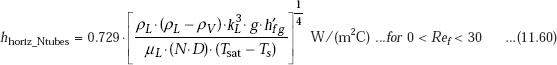
Average heat transfer coefficient for film condensation on a vertical tier containing N tubes is obtained by substituting (N.D) in place of D in Eq. 11.57 for a single horizontal tube, i.e.
Clearly, this is related to the value of heat transfer coefficient for a single horizontal tube as follows:
Vertical Tier of N Horizontal tubes:
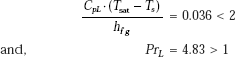
Chen (1961) has suggested the following modified form of Eq.11.57 for condensation on a vertical tube bank, to take into account the condensation occurring on the sub-cooled film between two adjacent tubes:
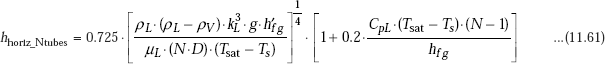
Note that the second square brackets on the RHS, is a correction factor to Eq. 11.60; also note that term inside this square bracket is hfg and not h’fg. Eq. 11.61 is valid for:
and,
11.4.5 Effect of Vapour Velocity, Nature of Condensing Surface and Non-condensable Gases
Effect of vapour velocity:
Above formulas are valid for stationary vapour or vapour moving at very low velocities (V < 10 m/s). At higher velocities, there will be friction between the liquid film and moving vapour. For a vertical plate, if the vapour is moving upwards, it will act to decrease the film velocity since the film is moving downwards and so, the film thickness will increase and the heat transfer coefficient will decrease. When the frictional force overcomes the gravity force, the film will get detached from the surface and the heat transfer coefficient will increase. Instead, if the vapour moves downwards in the direction of motion of the liquid film, then the film velocity increases, film thickness decreases, and as a result, the heat transfer coefficient increases. It is also observed that at low pressures, effect of vapour velocity on heat transfer coefficient is small.
Effect of nature of condensing surface:
For a rough surface, or for a surface covered with an oxide film, the surface offers additional resistance to the flow of the film, thus increasing the thickness of the liquid film. This results in reduction of heat transfer coefficient.
Effect of non-condensable gases:
If the vapours contain air or other non-condensable gases, heat transfer coefficient reduces drastically. This happens because, only the vapours condense on the surface, and the non-condensable gases form a ‘cloud’ near the surface impeding the approach of vapours to the surface for further condensation. In connection with steam condensers, practical data indicate that even a one per cent of air (by mass) in the vapour causes a reduction of about 60% in the value of heat transfer coefficient. So, in industrial condensers, provision is made for continuous venting of the non-condensables from the system.
11.4.6 Simplified Calculations for Water
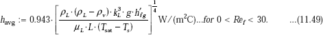
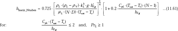
With reference to industrially important steam condensers, water vapour is condensed on the outside of tubes arranged mostly in a horizontal orientation. Then, for a horizontal tube, we have:
Then, without the correction for liquid sub-cooling, and for ρL >> ρV, we can write:
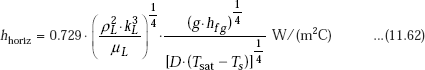
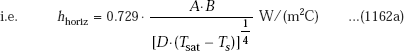
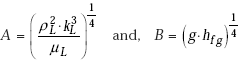
where,
For N horizontal tubes in a vertical tier, D in Eq. 11.62a is replaced by (N.D).
For vapours condensing on a vertical tube, again, Eq. 11.62a can be used, but with the modification that numerical constant 0.729 is replaced by 1.13 and D is replaced by the height of the tube, L.
Here, parameter A is evaluated at the mean film temperature {= (Tsat + Ts)/2} and parameter B is evaluated at Tsat.
Values of A and B can be conveniently tabulated for water for different values of Tsat and Ts, respectively. For the industrially important case of a steam condenser, Eq. 11.62a can be used to make a quick estimate of the heat transfer coefficient; values of parameters A and B can be read from Table 11.5 and Table 11.6, respectively, or from Fig. 11.10 and Fig. 11.11, respectively.
Example 11.9. Saturated steam at atmospheric pressure condenses on a vertical plate (size: 30 cm × 30 cm) maintained at 60°C. Determine heat transfer rate and the mass of steam condensed per hour.
(b) If the plate is tilted at an angle of 30 deg. to the vertical, what is the value of condensation rate?
Solution.
Data:
L := 0.3 m b := 0.3 m Tsat := 100°C Ts := 60°C and, Tf := 80°C (mean film temperature = (100 + 60)/2)
Properties of liquid at Tf = 80°C:
ρL := 971.8 kg/m3 CpL := 4197 J/kg.C μL := 0 355 × 10−3 kg/(ms) kL := 0.67 W/(mC) g := 9.81 m/s2
Properties of saturation vapours at 100°C:
hfg := 2257 × 103 J/kg ρV := 0.5978 kg/m3
Average heat transfer coefficient:
Let us assume laminar film condensation; we shall check this later.
Then, we have:
TABLE 11.5 Values of parameter ‘A’ at different mean film temperatures for water
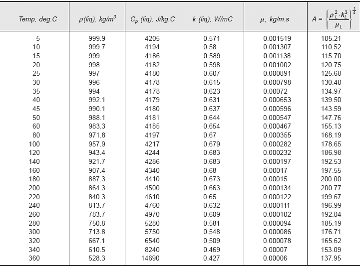
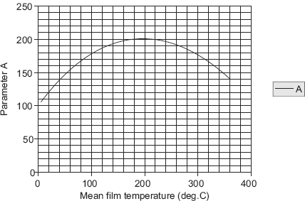
FIGURE 11.10 Parameter A for water
and,
i.e. havg = 5.917 × 10³ W/(m2C) (average heat transfer coefficient for the plate)
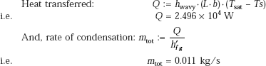
Heat transfer rate:
Q := havg · (L · b · (Tsat − Ts), W
i.e. Q = 2.13 × 10⁴ W (heat transfer rate to the plate)
Condensation rate of steam:
Now, check the assumption of laminar film condensation:
We have, film Reynolds number, given by:
where, P = wetted perimeter = b, for vertical plate
However, Ref is > 30; therefore, it is laminar-wavy region.
So, let us assume that condensation is laminar up to a particular distance L1 from top, and then it becomes wavy. Let us find out the distance from top, where film becomes wavy.
where, Q1 is the heat transfer to the plate up to the length L1
TABLE 11.6 Values of parameter ‘B’ at different saturation temperatures for water
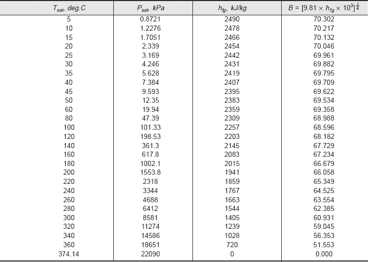
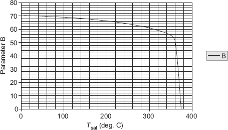
FIGURE 11.11 Parameter B for water
Then, from Eq. a:
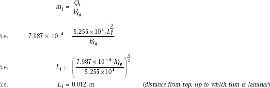
Therefore, length of plate over which film is wavy = L2 = 0.3 – L1
i.e. L2 = 0.288 m
Over the length L2, we use equation applicable to wavy film, namely.
where, by definition, Condensation number is:
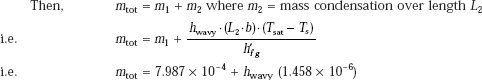
Let the rate of condensation over the total length of the plate be mtot:
Now, film Reynolds number for wavy region:
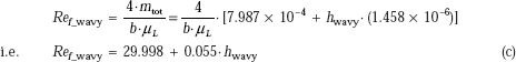
Then, from Eq. 11.50b and 11.52 and Eq. c we get:
Solve this for hwavy using solve block of Mathcad:
Start with a guess value for hwavy. Then, immediately after ‘Given,’ write the constraint equation Then, type the command “Find (hwavy)” and it is calculated immediately:
Given
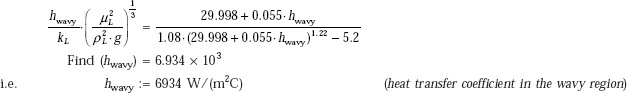
Now, from Eq. c:
Ref_wavy := 29.998 + 0.055 · hwavy …(c)
i.e. Ref_wavy = 411.368 < 1800, and > 30 (therefore, within the wavy region.)
Therefore, use of Eq. 11.52 for wavy region is justified.
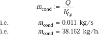
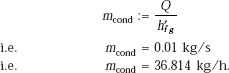
Then, total rate of condensation:
mtot := 7.987 × 10⁻⁴ + hwavy · (1.458 × 10⁻⁶)
i.e. mtot = 0.011 kg/s
i.e. mtot · 3600 = 39.27 kg/h (total rate of mass condensation.)
Comments: Above procedure, wherein we took into account the small, initial length from top of the plate where the film is laminar, is quite accurate. But, note that laminar film exists only for a distance of 0.012 m from top, whereas for the remaining 0.288 m of height, the flow is laminar-wavy.
So, if we make an approximation that the flow is laminar-wavy for the entire height of the plate, we get:
Note that this value of mtot is practically the same as obtained earlier with exact analysis. Therefore, it appears that calculations made assuming that the entire plate has laminar-wavy film, involve negligible error, with the advantage that the calculations are much easier to make.
Assuming that the film is laminar-wavy over the entire length of plate, calculations would proceed as follows:
Using the calculation formulas for laminar-wavy film region:
Laminar-wavy Reynolds number:
Now, since ![]() we write:
we write:
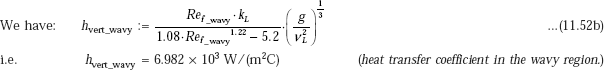
Heat transfer coefficient in laminar-wavy region:
Compare this value with the value of 6934 W/(m2C) obtained earlier with exact analysis.
Heat transferred:
and, rate of condensation:
(b) If the plate is tilted at 30 deg. to vertical:
We can determine h by replacing g by g.cos (θ) in equation for vertical plate.
Since h is already determined for vertical plate, we can use the relation:
Note: while using Mathcad, for trigonometric functions, θ must be expressed in radians:
Therefore,
and
Heat transferred:
and, rate of condensation:
i.e. for an inclined plate, rate of condensation is decreased by about 3.5% as compared to that on a vertical plate.
Example 11.10. Saturated steam at a temperature of 65°C condenses on a vertical surface at 55°C. Determine the thickness of the condensate film at locations 0.2 m and 1.0 m from top. Also, calculate the condensate flow rate, local and average heat transfer coefficients at these locations.
Properties of water at the mean temperature are:
(M.U. 2002)
Data:
ρL := 983.3 kg/m3 kL := 0.654 W/(mK) μL := 4.67 × 10⁻⁴ kg/(ms) CpL := 485 J/(kgC)
hfg := 2346 × 103 J/kg Tsat := 65°C Ts := 55°C g := 9.81 m/s2 b := 1 m (width, assumed)
Solution. Thickness of condensate film:
We have, from Eq. 11.43
When ρL >> pV we can write:
Therefore,
Mass flow rate of condensate:
We have, from Eq. 11.39:
Again, when ρL >> ρV we can write:
Therefore,
m(0.2) = 7.262 × 10⁻³ kg/s (mass flow rate of condensate at 0.2 m from top)
and, m(1.0) = 0.024 kg/s (mass flow rate of condensate at 1.0 m from top)
Heat transfer coefficients:
We can use Eq. 11.44 or 11.45. Since δ is already calculated, it is easier to use Eq. 11.44:
Again, writing hx as a function of x, Eq. 11.44 is re-written as:
Then,
hx(0.2) = 6.389 × 10³ W/(m2C) (local heat transfer coefficient at 0.2 m from top)
and, hx(1.0)= 4.272 × 10³ W/(m2C) (local heat transfer coefficient at 1.0 m from top)
Further, average heat transfer coefficient between x = 0 and x = x is given by Eq. 11.47, i.e.
We re-write this as:
Therefore,
havg(0.2) = 8.518 × 10³ W/(m2C) (average heat transfer coefficient between x = 0 and x = 0.2)
and, havg(1.0) = 5.697 × 10³ W/(m2C) (average heat transfer coefficient between x = 0 and x = 1.0 m)
McAdams has suggested that this calculated value of havg should be increased by 20% to account for liquid sub-cooling, i.e.
havg(1.0) = 1.2 × 5697 = 6846.4 W/(m2C) (corrected average heat transfer coefficient between x = 0 and x = 1.0 )m.
Note: All the above calculations have assumed that the film is purely laminar during condensation.
(b) In addition, if the height of the plate is 1 m let us calculate the following:
- heat transfer rate to the plate,
- maximum velocity of condensate at the trailing edge, and
- also, draw the variation of δ with distance from top.
Let us check if the condensation is of laminar type:
We should find film Reynolds number.
From Eq. 11.32 we have:
m has already been calculated as 0.024 kg/s at a distance of 1 m from top.
Note: However, note that Ref > 30; therefore, flow is really in the laminar-wavy region.
Assuming that the film is laminar-wavy over the entire length of plate, calculations would proceed as follows:
Using the calculation formulas for laminar-wavy film region:
We have:
Laminar-wavy Reynolds number:
Now, since ![]() we write:
we write:
i.e. Ref_wavy = 235.355 (Laminar–wavy Reynolds number)
Heat transfer coefficient in laminar-wavy region:
Note: Compare this value with the value of 6836.4 W/(m2C) obtained earlier for pure laminar film.
(i) Heat transfer rate:
Q := hvert_wavy · (L · b) · (Tsat − Ts) W
i.e. Q = 6.445 × 10⁴ W (heat transfer rate to the plate.)
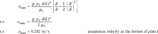
(ii) Maximum velocity of condensate at the bottom (i.e. trailing edge of plate):
Velocity is given by:
Now, the maximum velocity occurs when y = δ.
Therefore, remembering that ρL >> ρV we can write for maximum velocity at the bottom of the plate, i.e. at x = L, where δ = δ (L):
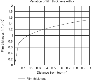
(iii) Draw the variation of δ with the distance from the top of the plate, x:
It is convenient to use Mathcad to draw this graph:
x := 0, 0.05, …, 1.0 (define a range variable x varying from x = 0 to x = 1 m at an interval of 0.05 m.)
Then, to draw the graph, click on the graph pallete, choose x–y graph, fill up the place holder on x-axis by x, and place holder on y-axis by [δ(x). 104) Click anywhere outside the graph area, and the graph appears:
Verify that at x = 1 m, δ is equal to 1.531 × 10⁻⁴, as already calculated. It is observed that film thickness is zero at x = 0, i.e. the top edge and goes on increasing with increasing x, i.e. as one travels down the plate.
Example 11.11. Dry, saturated steam at atmospheric pressure condenses on a horizontal tube of diameter = 5 cm and length L = 1 m; surface of the tube is maintained at 60°C. Determine heat transfer rate and the mass of steam condensed per hour. Assume laminar film condensation.
(b) If the tube is vertical, what is the condensation rate?
Solution.
Data:
Properties of liquid at Tf := 80°C:
ρL := 971.8 kg/m3 CpL := 4197 J/kgC μL := 0.355 × 10⁻³ kg/(ms) kL := 0.67 W/(mC) g := 9.81 m/s2
Properties of saturated vapour at 100°C:
(a) For horizontal tube:
We shall make a quick estimate using Eq. 11.62a:
where,
Now, A and B are to be evaluated at the mean film temperature (= 80°C) and at saturation temperature of steam (= 100°C), respectively. Value of A is read from Table 11.5 (or Fig. 11.10) and that of B from Table 11.6 (or Fig. 11.11). We get:
A := 168.19
and, B := 68.596
Therefore,
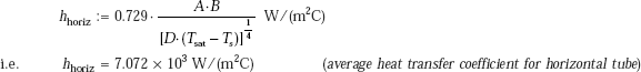
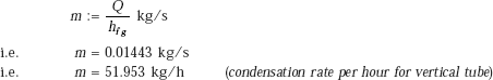
Heat transfer rate:
Q := hhoriz · (π · D · L) · (Tsat − Ts) W
i.e. Q = 4.444 × 10⁴ W (heat transfer rate to the tube.)
Condensation rate of steam:

(b) For vertical tube:
We shall make an estimate of ‘h’ using Eq. 11.62a. Since that equation is for horizontal tubes, we should change the numerical constant to 1.13, and D to L, to apply for vertical tubes:
Values of A and B are already determined:
i.e. A := 168.19
and, B := 68.596
Therefore,
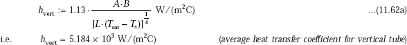
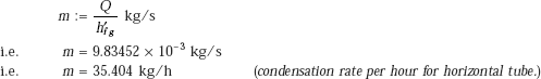
Heat transfer rate:
Q := hvert · (π · D · L) · (Tsat − Ts) W
i.e. Q = 3.257 × 10⁴ W (heat transfer rate to vertical tube.)
Condensation rate of steam:
Ratio of condensation rates:
i.e. amount of steam condensed on a horizontal tube is 36.4% more as compared to the amount condensed for a vertical tube.
Note: In the above analysis, effect of liquid sub-cooling has been neglected; also, laminar film condensation is assumed.
Example 11.12. Dry, saturated steam at atmospheric pressure condenses on a vertical tube of diameter = 5 cm and length L = 1.5 m; surface of the tube is maintained at 80°C. Determine the heat transfer rate and the mass of steam condensed per hour.
Solution.
Data:
Properties of liquid at Tf := 90°C
ρL := 965.3 kg/m3 CpL := J/kgC μL := 0.315 × 10⁻³ kg/(ms) kL := 0.675 W/(mC)
PrL := 1.96 g := 9.81 m/s2
Properties of saturated vapour at 100°C:
To start with, we shall assume that the film thickness δ << D, the tube diameter and also that the condensation is in pure laminar region; we shall check these assumptions later.
For laminar film condensation on vertical surface, we have:
i.e. havg = 4.83 × 10³ W/(m2C)
Heat transfer rate:
Condensation rate of steam:
Now, let us check the assumptions:
Film thickness δ:
We have, from Eq. 11.43:
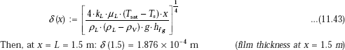
i.e. film thickness at the bottom end of the tube = 0.1876 mm << 5 cm. Therefore, the condition that δ << D is satisfied.
Next, let us check if film—Reynolds number is < 30:
Reynolds number:
We have:
where, P = wetted perimeter, i.e.
However, Ref > 30; so, it is in the laminar-wavy region. So, let us make calculations for laminar-wavy region:
Laminar-wavy region:
We have:
Calculation formulas for laminar-wavy region, for vertical plate/cylinder are:
Assuming that film on the entire tube length is laminar-wavy (see comments in Example 11.9),
Heat transferred:
And, rate of condensation:
Note: Let us compare the value of heat transfer coefficient for the wavy region, obtained above using Eq. 11.52b with that obtained using Chen’s correlation 11.54:
From Chen’s correlation:
This value, when compared to the value of 6160 W/(m2C) obtained earlier, is about 11.9% higher.
Example 11.13. A steam condenser consists of a square array of 400 horizontal tubes, each 6 mm in diameter. The tubes are exposed to exhaust steam arriving from the turbine at a pressure of 0.1 bar. If the tube surface temperature is maintained at a temperature of 25°C by circulating cold water through the tubes, determine the heat transfer coefficient and the rate at which the steam is condensed per unit length of tubes for the entire array. Assume laminar film condensation and that there are no condensable gases mixed with steam.
Solution.
Data:
![]() i.e. N := 20 L := 1.0 m D := 0.006 m Tsat := 45.8°C
i.e. N := 20 L := 1.0 m D := 0.006 m Tsat := 45.8°C
Ts := 25°C ∴Tf := 35.4°C (mean film temp.)
Properties of liquid at Tf = 35.4°C:
ρL := 994.04 kg/m3 CpL :=4178 J/kgC μL := 0.720 × 10⁻³ kg/(ms) kL := 0.623 W/(mC)
PrL := 4.83 g := 9.81 m/s2
Properties of saturated vapour at 45.8°C:
Then, for laminar film condensation on a vertical tier consisting of N horizontal tubes, we have
Therefore,
Heat transfer rate/m length:
Condensation rate of steam:

Then, for the entire array of 400 tubes, total condensation rate per metre length is:

Alternatively:
We an use Chen’s correlation for average heat transfer coefficient on a vertical tier of N horizontal tubes:
Let us check the conditions first:
Therefore, the conditions are satisfied.
Then, we have:
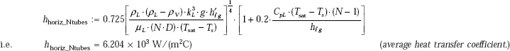
Compare this value with h = 5482 W/(m2C), obtained earlier from Eq. 11.60. We see that Chen’s correlation gives about 13.2% higher value of h.
Correspondingly, condensation rate also will be 13.2% higher:
11.4.7 Film Condensation inside Horizontal Tubes
Condensers used in vapour compression refrigeration and air-conditioning systems have refrigerant vapours condensing inside horizontal or vertical tubes. The situation is complicated to analyse and, obviously, heat transfer depends on vapour velocity.
For low vapour velocities, Chato recommends following correlation for condensation inside horizontal tubes, when the tube length is short or the rate of condensation is small:
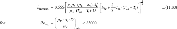
Reynolds number of vapours is evaluated at the inlet conditions, with the inside diameter of the tube as the characteristic length.
If the rate of condensation is high, or the tube is long, correlation of Ackers et al. may be used (with the understanding that error may be as high as 50%):
where, 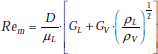
and, GL and GV are liquid and vapour mass velocities (kg/(m2s)) calculated on the basis of internal cross section of the tube (= π. D2/4). These correlations may be used for vapour Reynolds numbers > 20,000 and the liquid Reynolds number > 5,000.
Example 11.14. Ammonia at 40°C is condensing inside a horizontal tube of 16 mm ID. Mass velocity of ammonia vapour at inlet is 20 kg/(m2.s). Surface of the tube is maintained at a constant temperature of 20°C by circulating cold water. Calculate the fraction of vapour that will condense if the tube is 0.5 m long.
Solution.
Data:
L := 0.5 m D := 0.016 m GV := 20 kg/(m2s) Tsat := 40°C Ts := 20°C ∴ Tf := 30°C (mean film temp.)
Properties of liquid at Tf = 30°C:
ρL := 596.4 kg/m3 CpL := 4890 J/kgC μL := 2.081 × 10⁻⁴ kg/(ms) kL := 0.507 W/(mC) g := 9.81 m/s2
Properties of saturated vapour at 40°C:
hfg := 1098.8 × 103 J/kg ρV := 12.029 kg/m3 μV := 1.0735 × 10⁻⁵ kg/(ms)
Vapour Reynolds number:
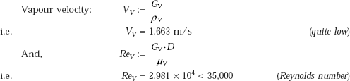
Therefore, we can use the correlation of Chato for film condensation inside a tube:
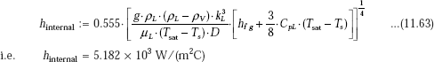
Then, rate of heat transfer:
Rate of condensation:
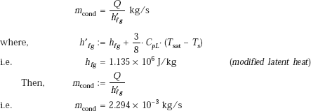
Rate of input of ammonia:
Therefore, fraction of vapour condensed:
i.e. 57.042% of the ammonia entering the tube is condensed over a length of 0.5 m.
11.4.8 Drop-wise Condensation
In drop-wise condensation, as already explained, heat transfer coefficient is higher (by as much as ten times) than that in film condensation, due to exposure of larger surface area to the vapours. Drop-wise condensation is achieved either by giving a coating of some material (such as teflon, gold, silver, rhodium, platinum, etc.) or by adding some promoting chemicals (such as waxes or fatty acids) to the vapours. However, maintaining the surface conditions favourable for drop-wise condensation is very difficult in practice, since these coatings lose their effectiveness in course of time due to fouling, oxidation, etc. In addition, the cost consideration also comes into picture.
Condensation of steam on copper surfaces has been studied extensively, because of its industrial importance (in Steam Power plants). P. Griffith recommends following simple correlations for drop-wise condensation of steam on copper surfaces:
It must be appreciated that in heat exchangers, it is the total thermal resistance to heat transfer that matters. Heat transfer coefficients are inherently high in boiling and condensation; so, the associated thermal resistance [= 1/(h.A)], is quite low. So, the heat transfer is more likely to be affected by other resistances such as the film resistance on the other side of the heat exchanger or the thermal resistance of the tube material. As such, it is not necessary to have an extremely high accuracy in the determination of heat transfer coefficients in boiling and condensation.
11.5 Summary
In this chapter, we studied two important phenomena that involve phase change, namely, boiling and condensation, which have great industrial importance.
When a liquid comes in contact with a heated surface maintained at a temperature Ts greater than the saturated temperature Tsat of the liquid at the given pressure, boiling occurs. Boiling phenomenon may be classified into two types: (a) pool boiling, and (b) flow boiling. In pool boiling, liquid remains stationary as in a ‘pool’ but for the convection currents caused by temperature differences and the heater is submerged in the liquid. In flow boiling, boiling occurs as the liquid flows past a heated surface or inside a heated tube.
In pool boiling, there are various boiling regimes depending upon the ‘excess temperature’, ΔTe (= Ts – Tsat). Since it is difficult to get analytical heat transfer correlations for boiling phenomenon, practical correlations are of empirical nature and such correlations for the different boiling regimes have been presented.
Flow boiling inside pipes is more complicated, because of the possibility of two-phase flow. Two of the practically important correlations for two-phase flow boiling have been presented along with those for nucleate flow boiling.
Condensation is of important relevance in steam condensers of thermal power plants. Condensation can be considered as the ‘reverse’ of boiling phenomenon. Again, condensation may be of two types: (a) film condensation, and (b) drop-wise condensation.
Film condensation may be of laminar or turbulent type. Nusselt’s relation for laminar film condensation on a vertical plate was derived. Several correlations for laminar film condensation on some other practically important geometries were presented. Concept of ‘condensation number’ and its use in correlations for laminar and turbulent film condensation correlations was explained. Some important data to quickly estimate the heat transfer coefficients for condensation of steam in a condenser were also given. Finally, for drop-wise condensation, simple correlations of Griffith for steam condensing in a drop-wise manner on copper surfaces were given.
Questions
- Differentiate between:
- evaporation and boiling
- sub-cooled boiling and saturated boiling, and
- pool boiling and flow boiling.
- With the aid of a neat sketch of a boiling curve for water (for pool boiling), explain the various regimes of boiling. [M.U.]
- Differentiate between nucleate boiling and film boiling. [M.U.]
- Draw the boiling curve for pool boiling of water and show the ‘burnout point’. What is its significance?
- What are the different flow regimes occurring in a vertical tube during flow boiling?
- Mention a few industrial applications where boiling and condensation are important.
- Differentiate between film condensation and drop-wise condensation. In which case is the heat transfer higher? Why?
- What is the mechanism of heat transfer in condensation? Using Nusselt’s theory, develop an expression for average heat transfer coefficient in condensation over a length of a vertical plate. [M.U.]
- What are the important assumptions in Nusselt’s theory of condensation on a vertical plate?
- What is ‘modified latent heat of vaporisation’? What is the purpose of introducing this quantity?
- Define ‘film—Reynolds number’. At what value of film Reynolds number does the condensate film flow become turbulent?
- Define ‘condensation number’. Draw a qualitative graph of film Reynolds number vs. condensation number, and identify the laminar, wavy and turbulent film flow regions.
- While calculating the film-Reynolds number, how is ‘wetted perimeter’ (P) defined?
- Show that the value of hydraulic diameter for film condensation on a vertical plate, vertical cylinder and a horizontal cylinder is given by: Dh = 4.δ, where δ is the film thickness.
- Considering the film condensation on horizontal and vertical tubes, in which case is the heat transfer coefficient higher? Explain.
- How is the average heat transfer coefficient in a vertical tier of N horizontal tubes related to the heat transfer coefficient for condensation on a single horizontal tube? In a given tier, where is the heat transfer maximum, for the upper tube or the tubes at the lower levels? Why?
- Write a short note on how the condensation heat transfer is affected by:
- nature of surface (smooth or rough)
- vapour velocity, and
- presence of non-condensable gases in the vapours.
Problems
- Water is boiled at atmospheric pressure in a mechanically polished, stainless steel pan of 30 cm diameter. Bottom surface of the pan is maintained at a temperature of 108°C. Calculate: (a) heat transfer coefficient (b) heat transfer rate, and (c) rate of evaporation of water.
- In Problem 1, (a) calculate the maximum heat flux and compare the nucleate boiling flux with the maximum heat flux (b) compare the values of heat transfer coefficient obtained from Rohsenow’s correlation with those obtained using Collier’s, Mostinski’s and Russian correlations.
- In problem 1 if the stainless steel pan is Teflon coated, how do the heat transfer coefficient and rate of evaporation change?
- A nickel wire, 1.5 mm diameter and 400 mm long, is submerged in a water bath open to atmosphere. What is the value of current flowing through the wire that will cause burnout, if the applied voltage is 10 V?
- A horizontal, metal-clad heating element, 8 mm diameter, and of surface emissivity 0.9, is submerged in a water bath. Surface temperature of the heating element is 340°C. If the water is at atmospheric pressure, calculate the power dissipation per unit length of the heater.
- A large, horizontal plate is kept immersed in a water bath boiling at 1 atm, 100°C. Surface temperature of the plate is 300°C. Calculate the heat transfer coefficient and the heat flux. Assume the emissivity of the surface as 0.85.
- Water is boiling at 7 atm. on the surface of a horizontal tube, whose wall temperature is maintained at 9°C above the boiling point of water. Calculate the nucleate boiling heat transfer coefficient.
(b) What is the change in the value of heat transfer coefficient when (i) temperature difference is increased to 18°C at the pressure of 7 atm., and (ii) pressure is raised to 14 atm. with ΔTe = 9°C?
- Water at 6 atm. flows inside a tube of 2.0 cm diameter under flow boiling conditions. Tube wall temperature is maintained at 7°C above the saturation temperature. Determine the heat transfer for one metre length of tube.
- A 50 mm diameter vertical evaporator tube (kw = 20 W/(mK)) carries 1 kg/s of steam at 11.71 bar (Psat = 460 K) at a quality x = 0.2. The tube is subjected to a uniform heat flux of 1.1 × 10⁶ W/m2. Identify the regime of flow boiling and calculate the convective heat transfer coefficient and surface temperature of the tube.
(b) When the quality reaches 0.8, what is the boiling regime and how much is the boiling heat transfer coefficient?
- In Problem 9, if the tube surface is maintained at a constant temperature of 227°C, calculate the total heat transfer coefficient and surface heat flux at the point where the quality is 0.2. Rest of the data are the same as in Problem 9.
- Saturated water at 1 atm. and velocity 1.5 m/s moves across a cylindrical heating element of 5 mm diameter. Find out the maximum heating rate for the element (W/m). [Hint: use the correlation of Lienhard and Eichhorn, Eq.11.21 or 11.22].
- Saturated steam at atmospheric pressure condenses on a vertical plate (size: 30 cm × 30 cm) maintained at 80°C. Determine heat transfer rate and the mass of steam condensed per hour. (b) If the plate is tilted at an angle of 30 deg. to the vertical, what is the value of condensation rate?
- Saturated steam at a temperature of 75°C condenses on a vertical surface at 65°C. Determine the thickness of the condensate film at locations 0.2 m and 1.0 m from top. Also, calculate the condensate flow rate, local and average heat transfer coefficients at these locations.
Properties of water at the mean temperature of 70°C are: ρL = 977.5kg/m3, kL = 0.663 W/(mK), μL = 0.000404 kg/(ms), CpL = 4190 J/(kgC). And, hfg at saturation temperature of 75°C = 2321 kJ/kg. Take ρV << ρL.
- In Problem 11.13, if the height of the plate is 1 m, calculate the following:
- heat transfer rate to the plate,
- maximum velocity of condensate at the trailing edge, and
- also, draw the variation of δ with distance from top.
- Dry, saturated steam at atmospheric pressure condenses on a horizontal tube of diameter = 3 cm and height L = 1 m; surface of the tube is maintained at 80°C. Estimate the heat transfer rate and the mass of steam condensed per hour. Assume laminar film condensation.
(b) If the tube is vertical, what is the condensation rate?
[Hint: Use Eq. 11.62a].
- Dry, saturated steam at atmospheric pressure condenses on a vertical tube of diameter = 5 cm and length L = 1.5 m; surface of the tube is maintained at 60°C. Determine the heat transfer rate and the mass of steam condensed per hour.
- A steam condenser consists of a square array of 625 horizontal tubes, each 6 mm in diameter. The tubes are exposed to exhaust steam arriving from the turbine at a pressure of 0.15 bar. If the tube surface temperature is maintained at a temperature of 25°C by circulating cold water through the tubes, determine the heat transfer coefficient and the rate at which the steam is condensed per unit length of tubes for the entire array. Assume laminar film condensation and that there are no condensable gases mixed with steam.
- A steam condenser consists of an array of horizontal tubes, each 2.0 cm in diameter and 1.5 m long. The tubes are arranged in such a manner that each vertical tier has 10 tubes; tubes are exposed to saturated steam at 100°C. If the tube surface temperature is maintained at a temperature of 80°C, determine the total number of tubes required to get a condensation rate of 0.4 kg/s. Assume laminar film condensation and that there are no condensable gases mixed with steam.
- Ammonia at 40°C is condensing inside a horizontal tube of 25 mm ID. Mass velocity of ammonia vapour at inlet is 10 kg/(m2s). Surface of the tube is maintained at a constant temperature of 20°C by circulating cold water. Calculate the fraction of vapour that will condense if the tube is 0.5 m long.
- In Problem 19, if ammonia is condensing on the outside surface of the tubes, what will be the heat transfer rate?