4
Approach for Estimating e-Waste Generation
Amit Kumar
University of British Columbia, NBK Institute of Mining Engineering, 6350 Stores Road, Vancouver, BC V6T 1Z4, Canada
4.1 Background
Estimation of the amount of e-waste generated every year is one of the challenging processes for designing any recycling or disposal practices. The success of an e-waste recycling or disposal facility depends on the annual throughput to plant. Without a constant throughput to the facility, the plant will have to go through larger downtime due to unavailability of the input feedstock. Hence, it is important to quantify the e-waste generation statistics accurately that in turn will help the recycling/disposal facilities to size their plant capacity and equipment dimensions properly to reduce the overall downtime. The proper estimation of e-waste generation in given region also helps understand the severity of the issue and helps the concerning authorities to formulate proper action plan to tackle the e-waste problem. There have been several studies to estimate the e-waste generation. This chapter lists the most common methods for predicting the total e-waste generated in any calendar year.
4.2 Econometric Analysis
Kusch et al. (2017) studied the relation of waste generation and gross domestic product (GDP) for 50 countries of the pan-European region. It was shown that GDP per capita adjusted for purchasing power parity (PPP) has a linear dependency with e-waste generated per capita (coefficient of determination: 0.7657). Removing Luxembourg (due to its small population and high GDP per capita) improved the coefficient of determination to 0.93.
Kumar et al. (2017) also showed that a linear relationship exists between the GDP and the amount of e-waste generated in a country, whereas no significant relation was observed between the population and the amount of e-waste produced by the country. It was also concluded that the electronic waste generated per inhabitant in any country was correlated with the per capita income of the inhabitants as shown in Figure 4.1. It shows that certain countries in Asia with relatively higher per capita income such as the United Arab Emirates, Qatar, and Japan produced more waste compared to other Asian countries with lower PPP such as India, Bangladesh, and Pakistan. The size of the marker in Figure 4.1 represents the population of the country. It suggests that e-waste generation is proportional to the purchasing power for any given country.

Figure 4.1 E-waste generated per capita with respect to the PPP and population.
Source: Data from Baldé et al. (2017) and World Bank (2019).
The econometric model is a regression-based model that uses various economic factors such as GDP, growth rate, population, PPP of an economy to estimate the e-waste generation (Yedla 2016). This method does not account for the consumer behavior, and the life span of electrical and electronic equipment (EEE).
4.3 Consumption and Use/Leaching/Approximation 1 Method
This method estimates an average e-waste generation based on the household stock of EEE and its average lifespan (L) assuming a saturated market where a fixed percentage of the stocked EEE will enter the waste stream every year. The stock data for a calendar year are estimated based on the number of households H(t), penetration/saturation level per capita or per household N(t), and the average weight (W) of the EEE. The e-waste generated in a calendar year can be calculated using Eq. (4.1) (Ikhlayel 2016).
However, this method also does not account for the life span distribution of EEE, rather it relies on the average lifetime of EEE.
4.4 The Sales/Approximation 2 Method
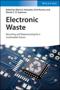
The sales method as defined by Bogar et al. (2019) or the Approximation 2 method as defined by UNEP (2007) uses sales statistics to estimate the total e-waste generated in a given year. It assumes a saturated market where e-waste in any given year is the same as the total new sales of electronics goods in the same year. Mathematically, it can be shown as Eq. (4.2).
However, this method also does not account for the consumer behavior and the life span distribution of EEE.
4.5 Market Supply Method
The market supply method uses sales of a given EEE and its lifespan to estimate the e-waste generation. The method can be subdivided into three categories that combine the probability of reuse, storage, and disposal along with the lifespan for all these levels to predict the total e-waste generation.
4.5.1 Simple Delay
This method assumes that an EEE will enter the waste stream at the end of its lifespan. If the life span of a given product is “L” year, then that product will enter in the waste stream “n” year after the purchase. Mathematically, it can be shown as Eq. (4.3) (Bogar et al. 2019).
However, this method also does not account for the consumer behavior and the variation of life span of EEE over the year.
4.5.2 Distribution Delay Method
The distribution delay method is a more accurate version of the simple delay method. It considers the probability of an EEE to enter the waste stream. The lifespan of a given product is not averaged but used in a probabilistic form (Miller et al. 2016; Wang et al. 2013). Weibull distribution is most widely used to determine the probabilistic obsolescence rate in any given year (Polák and Drápalová 2012) and will be discussed in Section 4.9 in detail. The amount of e-waste generated in any given year can be estimated using Eq. (4.4).
where,
- t is the year for which e-waste quantity is being determined
- to is the base year (year the product was sold)
- L(p) (i, t) is the lifetime profile of EEE in a given year
4.5.3 Carnegie Mellon Method/Mass Balance Method
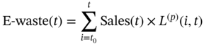
Carnegie Mellon method is a more detailed version of the simple delay method that uses different disposal levels of an EEE. It also uses different lifespans for these disposal scenarios and applies a percentage to estimate the movement of a product to one phase to the other phase and thus provide high accuracy. Different phases of products are reuse, storage, recycle, and landfill. It uses comprehensive material flows and their respective lifetime (Bogar et al. 2019; Wang et al. 2013). It requires a separate analysis for each product life phase. The e-waste generation can be determined using Eqs. (4.5)–(4.9) (Bogar et al. 2019; Miller et al. 2016).

where,
- The lifespan of the product for first use is L, reuse is Lr, and store is Ls.
- t is the year for which e-waste quantity is being determined.
- P1 to P9 is the disposal percentages of obsolete reused, obsolete stored, obsolete recycled, obsolete landfilled, reused stored, reused recycled, reused landfilled, stored recycled, and stored landfilled, respectively.
4.6 Time-Step Method
The time-step method calculates the amount of e-waste generated based on the sales and stock data of EEE. E-waste amount in a calendar year is estimated by the difference between the sales of EEE in the current year and the change in EEE stock in previous two years (Bogar et al. 2019; UNEP 2007; Wang et al. 2013). The method can be shown as Eq. (4.10).
Table 4.1 Methods to estimate e-waste generation.
| Required data | Market type | |||||
|---|---|---|---|---|---|---|
| Method | Sales | Stock | Lifespan | Saturated | Dynamic | Accuracy |
| Econometric analysis | Low | |||||
| Consumption and use | X | X | X | Low | ||
| Sales method | X | X | Low | |||
| Simple delay | X | X | X | Medium | ||
| Distribution delay | X | X | X | X | High | |
| Carnegie Mellon | X | X | X | X | X | High |
| Timestep | X | X | X | X | High | |
Sources: Based on Chancerel (2010), Ikhlayel (2016), Polák and Drápalová (2012), UNEP (2007), and Wang et al. (2013).
4.7 Summary of Estimation Methods
There are various methods available to estimate the amount of e-waste generated in a given year. The applicability of these methods depends on the quality of available data. Most of these methods are based on the sales and stocks of EEE and consumer behavior. The reliability of these data for a given time frame and for a country will be different, and it will also define the usefulness of the method. The summary of the listed methods, the input variables, and the level of accuracy are listed in Table 4.1.
4.8 Lifespan of Electronic Products
Most of the highly accurate methods listed in Table 4.1 require the average lifespan or the distribution of the lifespan of any given EEE. The lifespan of a product is the time it takes for any product to be discarded by its owner. The estimated lifespan of a few electronics products is listed in Table 4.2. It shows that the lifespan of consumer electronics has decreased in the past few years. Ala-Kurikka (2015a,b), Ely (2014), Geere (2015), Ahmed (2016), and Umweltbundesamt (2016) have all suggested a similar trend, which is a major reason of the increasing e-waste quantities around the globe.
As mentioned in the Carnegie Mellon method, a product might go through various phases such as storage and reuse before being discarded; hence, modeling a realistic lifespan is quite challenging. Thiébaud-Müller et al. (2018) used detailed social media and emailed surveys in Swiss households to obtain service lifetime and storage lifetime of 10 electronic devices. Oguchi (2015) listed three methods to estimate the lifetime distribution of products. The methods are based on survey data to obtain the discard rate distributions for different products. The survey would be conducted at the recycling or disposal facilities to collect the discard distributions, whereas a questionnaire to the consumers will provide information about the duration of use/reuse and domestic service lifetime. Oguchi et al. (2016) used these survey methods to estimate the lifespan of several types of EEE.
Table 4.2 Estimated lifespan of EEE.
| Average lifespan | ||
|---|---|---|
| Items | Ely (2014) | Abbondanza and Souza (2019) |
| Flat-panel TV | 7.4 | 4.3 |
| Desktop computer | 5.9 | 5.9 |
| Laptop | 5.5 | 4.0 |
| Cellphones | 4.7 | 2.3 |
| Smartphones | 4.6 | 1.8 |
| Refrigerator | — | 7.8 |
| Washing machine | — | 6.8 |
| Basic printer | — | 2.9 |
Santoso et al. (2019) suggested that the lifespan of a product can be classified into two types: average lifespan, which is often used in estimating e-waste in developing countries due to unavailability of data or unreliable data and distribution lifespan that provides more detailed lifespan but is difficult, time consuming, and expensive. A simplified method to obtain the distribution of lifespan is to use Weibull distribution with the Weibull lifespan and a distribution factor (Baldé et al. 2017; Environmental Protection Agency 2016; Miller et al. 2016; Oguchi and Fuse 2015; Polák and Drápalová 2012; Santoso et al. 2019; Sumasto et al. 2019; Tran et al. 2016).
Polák and Drápalová (2012) detailed the method to estimate the Weibull lifespan and the distribution factor using the lifespan data based on the survey results of 2008. Baldé et al. (2015a) and the Environmental Protection Agency (2016) have used this method and listed the Weibull lifespan and the distribution factor of various EEE. The values provided by Baldé et al. (2015a) have further been used to estimate the e-waste generation around the globe in 2014, 2016, and 2019 (Baldé et al. 2015b, 2017; Forti et al. 2020).
4.9 Global e-Waste Estimation
The global e-waste generation data are published as the Global E-waste Monitor. It is a collaboration between the International Telecommunication Union, the Sustainable Cycles Program that is cohosted by the United Nations University and the United Nations Institute for Training and Research, and the International Solid Waste Association. It provides the e-waste estimates around the world. The method for the e-waste estimates is published by Forti et al. (2018).
For the purpose of the measurement, the products are classified in groups labeled as UNU-KEYS with comparable average weights, material composition, end-of-life characteristics, and lifetime distributions. The full list along with their respective Harmonized System (HS) codes is presented in the document published by Forti et al. (2018). Harmonized System (HS) codes are commonly used for the purpose of import–export around the world.
The amount of total e-waste generated for each product in every category is estimated using the Distribution delay method as described in Section 5.5. It uses the amount of a product placed in the market in a given year along with the lifetime distribution of that product as shown in Eq. (4.11).

where,
- n is the year for which e-waste quantity is being determined
- POM(t) is the product sold (put-on-market) in a given year t
- to is the base year (year the product was sold)
- L(p) (t, n) is discard-based lifetime profile of EEE sold in the year t
If the amount of a product placed/sold in the market is unknown, the POM can be estimated using Eq. (4.12) and domestic production, import and export information. If the domestic production is unknown, it is assumed to be zero. In case of imports and exports, the number of units of the product is converted to weight by using unit weight of products reported by Forti et al. (2018).
Some corrections are needed for the outliers of the POM data. These corrections are needed if
- The POM value is too low, most likely due to unavailability of the domestic production data for a country where domestic production would be relatively large.
- The POM value is too high, mostly likely due to the misrepresentation of the reporting codes or units.
- The POM value is too high, mostly due to an obsolete product that is not manufactured anymore.
A more realistic value for POM is obtained either by using historic values or from a comparable country and then used for estimation purposes.
To account for the e-waste produced from product placed in market prior to the current year, the POM data are also estimated for past year based on available data or market trend. The future POM values are also predicted using the past, current, and future forecast of the PPP of the country provided by the world economic outlook and its ratio with the past and current POM.
The next step of estimating the e-waste generated is to estimate the lifetime distribution of the electrical and electronic products. Researchers have shown that the Weibull distribution is the most suitable probability distribution function to model the discard behavior of EEE (Baldé et al. 2017; Environmental Protection Agency 2016; Miller et al. 2016; Oguchi and Fuse 2015; Polák and Drápalová 2012; Santoso et al. 2019; Sumasto et al. 2019; Tran et al. 2016).
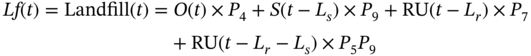
The simplified Weibull distribution of product discard-based lifetime profile is shown in Eq. (4.13) (Forti et al. 2018). The equation is mostly used for stable product with time independent lifetime. For these products, the variation in the shape and scale parameter is negligible overtime. The shape and scale parameters for various products are listed by Forti et al. (2018). The discard-based lifetime echoes the probability of an EEE entering the waste stream in a given year after its sale.
where,
- L is the lifetime profile of an EEE product sold in a base year t
- α is the distribution parameter, also known as the shape parameter
- β is the average lifespan, also known as the scale parameter
- n is the year for which the lifespan is being modeled
Figure 4.2 shows a sample plot for the discard probability and cumulative discard probability of various EEE using Eq. (4.13).
However, due to the technological developments (for example CRT screens), the lifetime of a EEE product could be time dependent meaning that the shape and scale parameters would change significantly overtime and the variations could not be neglected. In that case, the lifetime profile has to be modeled for each sales year using Eq. (4.14).
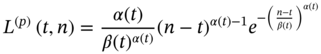

Figure 4.2 (a) Discard probability. (b) Cumulative discard probability of various EEE over their lifetime.
where,
- α(t) is the time-varying distribution parameter
- β(t) is the time-varying scale parameter
In terms of e-waste collection, the total amount of e-waste generated is also the combination of e-waste collected through various programs and e-waste discarded can be represented by Eq. (4.15).
where,
- Wformal is the e-waste collected by formal system, Wother is the e-waste collected by other recycling streams, Wbin is the e-waste discarded in bins, and Wgap is the quantity for which the fate of e-waste is unknown.
After the understating of e-waste generation and collection, the e-waste collection rate could be estimated using Eq. 4.16.
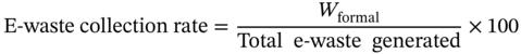
The European Union Directive 2012/19/EU (2012) provided e-waste collection and recycling targets for member countries. They enforced an 85% collection and 80% reuse/recycling target for e-waste categories 1 and 4, 80% collection and 70% reuse/recycling target for e-waste category 2, 75% collection and 55% reuse/recycling target for e-waste categories 5 and 6, and 80% reuse/recycling target for e-waste category 3 from 15 August 2018.
References
- Abbondanza, M.N.M. and Souza, R.G. (2019). Estimating the generation of household e-waste in municipalities using primary data from surveys: a case study of Sao Jose dos Campos, Brazil. Waste Management 85: 374–384. https://doi.org/10.1016/J.WASMAN.2018.12.040.
- Ahmed, S. F. (2016). The global cost of discarded electronics waste. https://www.theatlantic.com/technology/archive/2016/09/the-global-cost-of-electronic-waste/502019 (accessed 17 March 2021).
- Ala-Kurikka, S. (2015a). Electronic goods’ life spans shrinking, study indicates. http://www.endseurope.com/article/39711/electronic-goods-life-spans-shrinking-study-indicates (accessed 17 March 2021).
- Ala-Kurikka, S. (2015b). Lifespan of consumer electronics is getting shorter, study finds. https://www.theguardian.com/environment/2015/mar/03/lifespan-of-consumer-electronics-is-getting-shorter-study-finds (accessed 17 March 2021).
- Baldé, C. P., Forti, V., Gray, V., Kuehr, R., and Stegmann, P. (2017). The global e-waste monitor – 2017. https://www.itu.int/en/ITU-D/Climate-Change/Documents/GEM2017/Global-E-waste Monitor 2017.pdf (accessed 17 March 2021).
- Baldé, C. P., Kuehr, R., Blumenthal, K., et al. (2015a). E-waste statistics – Guidelines on classification, reporting and indicators. http://collections.unu.edu/view/UNU:5620 (accessed 17 March 2021).
- Baldé, C.P., Wang, F., Kuehr, R., and Huisman, R. (2015b). The global e-waste monitor-2014. https://i.unu.edu/media/unu.edu/news/52624/UNU-1stGlobal-E-Waste-Monitor-2014-small.pdf (accessed 17 March 2021).
- Bogar, Z.O., Capraz, O., and Güngör, A. (2019). An overview of methods used for estimating E-waste amount. In: Electronic Waste Management and Treatment Technology (eds. M.N.V. Prasad and M. Vithanage), 53–75. Butterworth-Heinemann, Elsevier https://doi.org/10.1016/B978-0-12-816190-6.00003-0.
- Chancerel, P. (2010). Substance Flow Analysis of the Recycling of Small Waste Electrical and Electronic Equipment: An Assessment of the Recovery of Gold and Palladium. Berlin: Institut für Technischen Umweltschutz.
- Ely, C. (2014). The life expectancy of electronics. http://www.cta.tech/Blog/Articles/2014/September/The-Life-Expectancy-of-Electronics (accessed 17 March 2021).
- Environmental Protection Agency (2016). Electronic products generation and recycling in the United States, 2013 and 2014. https://www.epa.gov/smm/advancing-sustainable-materials-management-facts-and-figures-report (accessed 17 March 2021).
- Forti, V., Baldé, C. P., Kuehr, R., and Bel, G. (2020). Global E-waste monitor 2020: quantities, flows and the circular economy potential. https://www.itu.int/en/ITU-D/Environment/Documents/Toolbox/GEM_2020_def.pdf (accessed 17 March 2021).
- Forti, V., Baldé, K., and Kuehr, R. (2018). E-waste Statistics: Guidelines on Classifications, Reporting and Indicators, 2e. United Nations University http://collections.unu.edu/view/UNU:6477 (accessed 17 March 2021).
- Geere, D. (2015). Electronic product lifespans are getting shorter. www.wired.co.uk/article/product-lifespans.
- Ikhlayel, M. (2016). Differences of methods to estimate generation of waste electrical and electronic equipment for developing countries: Jordan as a case study. Resources, Conservation and Recycling 108: 134–139. https://doi.org/10.1016/J.RESCONREC.2016.01.015.
- Kumar, A., Holuszko, M., and Espinosa, D.C.R. (2017). E-waste: an overview on generation, collection, legislation and recycling practices. Resources, Conservation and Recycling 122: 32–42. https://doi.org/10.1016/j.resconrec.2017.01.018.
- Kusch, S., Hills, C.D., Kusch, S., and Hills, C.D. (2017). The link between e-waste and GDP – new insights from data from the Pan-European region. Resources 6 (2): 15. https://doi.org/10.3390/resources6020015.
- Miller, T.R., Duan, H., Gregory, J. et al. (2016). Quantifying domestic used electronics flows using a combination of material flow methodologies: a US case study. Environmental Science & Technology 50 (11): 5711–5719. https://doi.org/10.1021/acs.est.6b00079.
- Oguchi, M. (2015). Methodologies for estimating actual lifetime distribution of products. Product Lifetimes and the Environment, Nottingham Trent University, UK, 388–393. https://www.plateconference.org/methodologies-estimating-actual-lifetime-distribution-products.
- Oguchi, M. and Fuse, M. (2015). Regional and longitudinal estimation of product lifespan distribution: a case study for automobiles and a simplified estimation method. Environmental Science and Technology 49 (3): 1738–1743. https://doi.org/10.1021/es505245q.
- Oguchi, M., Tomohiro, T., Daigo, I., et al. (2016). Consumers’ expectations for product lifetimes of consumer durables. 2016 Electronics Goes Green 2016+, EGG 2016, 1–6. https://doi.org/10.1109/EGG.2016.7829850.
- Polák, M. and Drápalová, L. (2012). Estimation of end of life mobile phones generation: the case study of the Czech Republic. Waste Management 32 (8): 1583–1591. https://doi.org/10.1016/J.WASMAN.2012.03.028.
- Santoso, S., Yuri, M., Zagloel, T. et al. (2019). Estimating the amount of electronic waste generated in Indonesia: population balance model. IOP Conference Series: Earth and Environmental Science 219 (1): 012006. https://doi.org/10.1088/1755-1315/219/1/012006.
- Sumasto, F., Zagloel, T.Y.M., Ardi, R., and Zulkarnain (2019). Estimation lifespan of home electronic appliances in Indonesia: the case study of Java Island. IOP Conference Series: Earth and Environmental Science 219 (1): 012008. https://doi.org/10.1088/1755-1315/219/1/012008.
- The European Union (2012). Directive 2012/19/EU of the European Parliament and of the Council of the 4 July 2012 on waste electrical and electronic equipment (WEEE). Official Journal of the European Union L 197. https://eur-lex.europa.eu/legal-content/EN/TXT/PDF/?uri=CELEX:32012L0019&from=EN (accessed 17 March 2021): 38–71.
- Thiébaud-Müller, E., Hilty, L.M., Schluep, M. et al. (2018). Service lifetime, storage time, and disposal pathways of electronic equipment: a Swiss case study. Journal of Industrial Ecology 22 (1): 196–208. https://doi.org/10.1111/jiec.12551.
- Tran, H.P., Wang, F., Dewulf, J. et al. (2016). Estimation of the unregistered inflow of electrical and electronic equipment to a domestic market: a case study on televisions in Vietnam. Environmental Science & Technology 50 (5): 2424–2433. https://doi.org/10.1021/acs.est.5b01388.
- Umweltbundesamt (2016). Lifetime of electrical appliances becoming shorter and shorter. https://www.umweltbundesamt.de/en/press/pressinformation/lifetime-of-electrical-appliances-becoming-shorter (accessed 17 March 2021).
- UNEP (2007). E-waste Volume 1: Inventory Assessment Manual, 1e. United Nations https://wedocs.unep.org/bitstream/handle/20.500.11822/7857/EWasteManual_Vol1.pdf?sequence=3&isAllowed=y (accessed 17 March 2021).
- Wang, F., Huisman, J., Stevels, A., and Baldé, C.P. (2013). Enhancing e-waste estimates: improving data quality by multivariate input–output analysis. Waste Management 33 (11): 2397–2407. https://doi.org/10.1016/J.WASMAN.2013.07.005.
- World Bank (2019) Population, total. Available at: https://data.worldbank.org/indicator/sp.pop.totl (accessed 24 April 2019).
- Yedla, S. (2016). Development of a methodology for electronic waste estimation: a material flow analysis-based SYE-waste model. Waste Management & Research 34 (1): 81–86. https://doi.org/10.1177/0734242X15610421.