
Alternating current
An AC voltage or current is any which is changing. It will very often be one which changes at a known rate. Where a DC voltage or current is easily described by its magnitude and sign (‘3 V DC’ or ‘−16.2 V DC’ says it all, as long as we know where 0 V is), AC signals are a bit more complicated. We are going to start by considering the simplest type of AC signal. Then we will look at more complex ones.
The most ubiquitous AC signal is the sine wave. We will understand so much electronics in terms of how circuits respond to sine waves that it is worth our while spending some time describing and thinking about them.
The sine wave
If you haven’t known about sine waves before, the word ‘sine’ probably brings back dimly remembered memories of school maths lessons, trigonometry, and all that goes with it. The sine is a mathematical function which describes the ratio of two sides of a right angled triangle in relation to one of the other angles, and a sine wave is a graph of the ratio against the angle. That’s putting it mathematically. To many technicians and engineers, who try to do as much practical work as possible with the minimum use of mathematics, a sine wave is a very useful ‘wiggle’ which appears on the screens of an oscilloscope (a device which cleverly shows a graph of voltage against time) when they are working on equipment. We describe a great number of the essential properties of circuits in terms of what comes out when the input is a sine wave. The reasons for this are discussed later.
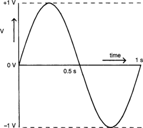
Figure 4.1 shows a sine wave. It is 2 V peak to peak (pk–pk or p-p) with a frequency of 1 Hz. (We’ll define these terms soon.) The voltage begins at a level of 0 V, rises smoothly up to a level of 1 V, back down through 0 V to −1 V, and up to 0 Vagain. Each transition, 0 V to 1 V, 1 V to 0 V, 0 V to −1 Vand−1 V to 0 V, takes the same amount of time, 0.25 s. The whole process is referred to as ‘one cycle’.
We don’t often come across sine waves which exist for one cycle only and then stop, however; usually the voltage oscillates continually while the circuit generating it is on. This may be for many hours. We call this a ‘continuous signal’.
There are two things that we need to describe a sine wave unambiguously; how big it is, and how long it takes to complete one cycle. These two quantities we normally call ‘amplitude’ and either ‘period’ or ‘frequency’.
Amplitude
There are three ways of defining the amplitude of a sine wave:
1. Peak to peak amplitude is the difference between the positive and the negative peaks. Figure 4.1 is a sine wave of 2 V pk–pk. Pk–pk amplitude can be used to describe signals which are not sine waves as well.
2. Peak amplitude is the difference between the mid-point of the signal and the positive peak. Figure 4.1 is a sine wave of (1–0) = 1 V pk. We can say that:
3. Root mean square (RMS) amplitude is the level of a DC signal which has the same energy content as the AC signal. This odd way of specifying amplitude exists because it is needed for power calculations (on which more later in this chapter). For a sine wave:
or:
or again:
Which of these three we use depends on the situation, and we often need to convert between them. For instance, we might see a sine wave displayed on the screen of our oscilloscope, and wish to calculate the power which it causes to be dissipated in a certain component. Here we might read the pk–pk amplitude from the display, divide by two to get pk amplitude and then multiply by 0.707 to get the RMS amplitude. Then we can make a power calculation. Conversely, we might measure the amplitude of a sine wave using an RMS multimeter. If we needed for some reason to have a rough idea of the pk–pk value of the voltage, we could divide by 0.7 (multiply by 1.4) and then multiply by 2 in our heads—multiply by 2.8.
Period and frequency
The period of a sine wave is the time which it takes to complete one cycle. Its symbol in equations is T, and its unit is that of time, the second (s). For Figure 4.1, T is one second.
It is more usual to refer to the ‘frequency’ of a sine wave. The symbol for frequency in equations is f, and its unit is the hertz, abbreviated to Hz, meaning cycles per second. The frequency is the number of cycles completed in one second. Converting from frequency to period is very easy:
with f in Hz and T in s.
So our signal of Figure 4.1 has a frequency of 1 Hz.
Amplitude and frequency are independent of each other; a sine wave of 3 kHz will oscillate 3000 times per second whether it has a level of 1μV or 10 V. One of 10 V RMS will still be at 10 V RMS, and have the same heating effect through a given resistor whether it is at 10 Hz or 1 MHz.
(An interesting aside to this second case; if the frequency were 0.01 Hz, a period of 100 s, would this still be true? No; remember, from Chapter 3, the mechanism of heating and cooling of resistive components. In this case, the frequency is so low that we would do better to consider it as a slowly varying DC voltage. For a quarter of the period, 25 s, the resistor will have a voltage across it of 20 V or greater! This time is obviously long enough to destroy the resistor if it is not adequately rated. In our power calculations, we should budget for the pk amplitude of about 14 V. This is a very extreme example, and such slow moving signals are not often encountered. The statement in the above paragraph holds true for frequencies of a few Hz and above.)
Phase
We can describe a single sine wave completely by specifying its amplitude and frequency. When we are talking about two such signals the important question of phase arises.
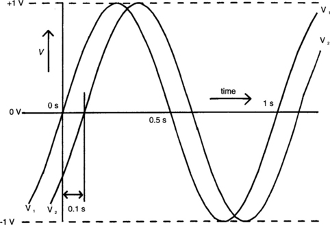
Figure 4.2 shows the sine wave of Figure 4.1 again, labelled V1, and a second nearly identical sine wave which starts its cycle at a later time t, labelled V2. We say that there is a phase difference between V1 and V2.
Phase is an angular quantity, and its units are degrees or radians. We use degrees in this book. There are two important points to bear in mind when talking about phase:
1. We only generally make phase comparisons between waveforms of the same frequency.
2. Phase, like voltage, is a relative quantity. It is meaningless to say that, for instance, ‘the voltage has a phase angle of 30°’ unless we specify that that 30° refers to some other waveform. A reference must be specified.
To calculate the phase difference between two waveforms, we use the following expression:
We can, of course, calculate t from ϕ and T:
where ϕ is the phase in degrees, t is the time difference in seconds and T is the period in seconds. For example, if t in Figure 3.2 is 100 ms, then ϕ = 36°. V2 starts 100 ms after V1, so we can either say that V2 lags V1 by 36° or that V1 leads V2 by 36°. The two statements mean the same thing. We might, if we were being awkward, say that V2 leads V1 by (360–36)° or 324°. This statement means that V2 starts its cycle 324°, or 900 ms, before V1 – just as true if they are continuous, but not the easiest way to say it. Normally we specify phase using the smallest possible angle, which is always less than 180°. Sometimes calculations give us numbers larger than this, and we convert them to a more sensible form.
Waveforms which are 90° out of phase are said to be in quadrature, while ones which are 180° out of phase are said to be in antiphase. Putting a waveform in antiphase is ‘inverting’ it. Waveforms which have no phase difference are simply ‘in phase’.
Calculations on AC quantities
We can do calculations on AC quantities of the same frequency to analyse the behaviour of a circuit at that frequency. Every quantity that we use will have two components; magnitude (amplitude) and phase.
Mathematical operations on waveforms of any phase are slightly tricky and require the use of something called ‘phasor mathematics’. Ideally, a mathematical technique called ‘complex algebra’ is used which makes use of a notional quantity called j, equal to ![]() to denote a phase shift of 90°. This technique allows not only voltages and currents but also combinations of reactances, resistances and even amplification to be treated under one umbrella. The behaviour of circuits can then be predicted at a fixed frequency.
to denote a phase shift of 90°. This technique allows not only voltages and currents but also combinations of reactances, resistances and even amplification to be treated under one umbrella. The behaviour of circuits can then be predicted at a fixed frequency.
The algebra involved is actually not much more difficult than the more conventional techniques which the next chapter uses, but a complete explanation of it is somewhat beyond the scope of this book. Should you already be familiar with it then Appendix 4 gives a quick restatement of its principle techniques.
Even if you are not (or don’t want to bother with it) its not really a problem. There are some simple rules and special cases of phasor mathematics which are presented below. In Part Three we will consider what some basic circuits do under these conditions and hence get a lot of insight into their workings. You could take these ideas on board now, or refer back to this point when you get there. Anyway, here goes:
Phase Rule 1: For waveforms in phase, magnitudes of quantities can be used in calculations directly. The phase of the result is the same as that of the ‘inputs’ to the calculation.
Phase Rule 2: A positive value of phase means ‘leading’, a negative one ‘lagging’.
Phase Rule 3: A negative value of magnitude means an inversion of the quantity (i.e. it is in antiphase). So subtraction is addition with one waveform inverted. We could say that – V is Vat an angle of 180°.
Phase Rule 4: Adding two equal waveforms in antiphase gives a result of zero. This is called ‘phase cancellation’.
Phase Rule 5: Multiplication of any pair of waveforms. The magnitudes are multiplied and the phase angles added together.
Phase Rule 6: Division of any pair of waveforms. The magnitudes are divided and the phase of the denominator subtracted from the phase of the numerator.
Resistors and sine waves
The terms pk, pk–pk and RMS can be used to refer to both voltages and currents. Provided that we are consistent we can do Ohm’s Law calculations on resistors with any of them. So, for example:
1. A pk voltage of 10 Vacross a 1k resistor causes a pk current of ![]() to flow.
to flow.
2. A pk–pk current of 3 mA through a 4k7 resistor causes a pk–pk voltage of 3 × 4k7 = 14.1 Vacross it.
3. An RMS voltage of 150 V across a 1M resistor causes an RMS current of ![]() to flow.
to flow.
Current and voltage through a resistor are always in phase. In fact, the current waveform is always an exact replica of the voltage waveform, its magnitude at every point being determined by Ohm’s Law.
Capacitors and sine waves
A capacitor with a sinusoidal voltage of frequency f across it will have a sinusoidal current flowing through it. The ratio of the voltage to the current is known as the ‘reactance’ of the capacitor at frequency f. The situation is analogous to that with a resistor, and the unit of reactance is again ohms. And Ohm’s Law again applies:
where XC is capacitive reactance, VC is the voltage across the capacitor and IC is the current through it. As with resistors, amplitudes of voltage and current can be specified using pk, pk–pk or RMS conventions, so long as the same is used for both.
We can calculate the reactance of a capacitor at any particular frequency using the expression:
where C is the capacitance in farads and f is the frequency. We can see from this that the magnitude of the reactance of a capacitor decreases proportionally with frequency.
But hold on! Capacitors are more than ‘frequency-dependent resistors’. They do something important to AC signals. The current through a capacitor always leads the voltage across it by 90°. This is the difference between a capacitor and a resistance with the same value as its reactance at that frequency.
We can often get a very good idea of what a circuit does by thinking of caps as ‘frequency-dependent resistors’, but we can’t do calculations to solve CR networks (using techniques from Chapter 5) without taking account of phase. (A CR network is any consisting of capacitors and resistors – we’ll meet CR, LR and LCR networks in Part Two.)
For calculation purposes, we consider that capacitive reactance has a phase angle of–90°, as passing a current with a phase angle of 0° through it results in a voltage of 90° lagging. (See Phase Rules 5 and 6 earlier in this chapter.) (It is this idea of assigning phase to reactance that makes otherwise incomprehensible complex numbers work.)
Now that we’ve met the terms resistance and reactance, this seems like the moment to mention the word ‘impedance’, which is used a lot. Strictly speaking, resistors have resistance, capacitors (and inductors) have reactance. Circuits have some combination of the two. If you want to be non-committal about which you mean, say ‘impedance’ – it can be either. And everyone should understand.
Inductors and sine waves
Like capacitors, the sinusoidal voltage across and current through an inductor are proportional at any given frequency. The ratio is again known as the reactance of the inductor, and here’s Ohm’s Law again:
with xL as inductive reactance, VL voltage across the inductor and IL current through it. Again we may use pk, pk–pk or RMS amplitudes but must be consistent. For an inductor voltage leads current by 90°, so we consider that the reactance has a phase angle of 90°. The inductive reactance can be calculated using the expression:
where L is the inductance in henries and f is the frequency in hertz. From this, inductive reactance increases proportionally with frequency.
(Again we see capacitors and inductors doing nice complementary things to each other, while resistors form a nice ‘neutral background’ against which to view it all.)
Why are sine waves so important?
In other words, why do we do so much of our analysis of AC circuits in terms of what they do when you put a sine wave through them?
All AC waveforms can be considered as being the sum of sine waves of various frequencies. The mathematical technique behind this is known as Fourier analysis. We are not going to get into the mathematics here, but we will consider the implications.
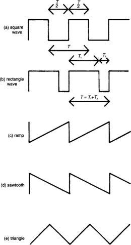
What the maths says is that we can treat any continuous periodic waveform (such as all the ones in Figure 4.3) as the sum of a number of sine waves of various frequencies. The frequencies will all be whole number multiples of the frequency of the repeating periodic waveform. So a 1 kHz triangle wave can be considered to be the sum of sine waves of 1 kHz, 2 kHz, 3 kHz … and so on. The amplitudes and phases of the sine waves will vary, generally getting less with frequency, but we could, if we knew them, and had the means to do it, reconstitute the waveform, like baking a cake to a recipe. For instance, the ‘recipe’ for a square wave of 1kHz is:
1 kHz sine wave, at 1 V RMS, plus …
3 kHz sine wave, at ![]() V RMS, plus …
V RMS, plus …
5 kHz sine wave, at ![]() V RMS, plus …
V RMS, plus …
’n‘can be any whole number as high as you care to keep going. The higher in frequency you continue, the better the shape of the resulting wave – that is the closer to the ideal, with the voltage changing from one voltage to the other almost instantaneously. Real square waves are not ideal, having a finite ‘risetime’ – the time taken to get from 10 to 90% of the value of the step.
You will notice in our square wave ‘recipe’ (known more properly as a Fourier series) that we only have the odd number multiples of 1 kHz. The 1 kHz waveform is known as the ‘fundamental’ of the series (i.e. the sine wave at the same frequency as the periodic waveform being analysed). The sine waves at 2 kHz, 3 kHz, and so on, are known as the ‘harmonics’ of the fundamental. 2 kHz would be the 2nd harmonic, 3 kHz the third, and so on. So we can say that ‘a square wave consists only of the fundamental plus odd harmonics’. It contains no even harmonics. The exact amplitude of the result can be foretold, but we are not often worried about it.
You can get tables showing the equations to write various waveforms in terms of their harmonics, but we rarely need them. Quite a lot can be done intuitively. Where a waveform has a sharp transition between two levels, that’s where you get the high harmonics. The ‘frequency response’ of a circuit is the way that its output, relative to the input, varies with frequency. If a circuit, such as a low-pass filter (of which more in Part Two) tends to attenuate high frequencies then it will affect the edges of a square wave – they will be slower. If we know the frequency at which the filter begins to ‘cut’, then we can get an idea of how serious this is – for example if our square wave is at 1 kHz, and the filter starts to ‘roll off’ from 2 kHz, the effect will be quite noticeable. If the filter rolls off from 20 kHz, much less so. Conversely, the low frequencies of a waveform contribute most to the portions where it changes slowly, or not at all; the top and bottom of a square wave will tend to ‘sag’. The time responses of 1st order circuits, which we look at in Chapter 9 are in fact extreme examples of this.
More AC waveforms
Figure 4.3 shows some types of AC signal which are commonly encountered. There is not too much to know about them, except to recognize their shapes and their names. With rectangle waves we sometimes hear talk of mark-to-space ratio. This is the ratio of duration of the more positive part to the more negative –T1 : T2 on the diagram. These waveforms are best specified, amplitude-wise, in terms of pk–pk level, again the difference between the positive and the negative voltage. Time-wise, we obviously refer to them by either their frequency or their period, with f = 1/T once again.
AC waveforms with a DC level
It often happens that we come across signals which are a combination of AC and DC. Then we say that the waveform has a ‘DC level’. The DC level of an AC waveform is just its average level. Hence if it has an equal area below 0 V as above it has a DC level of zero.
Sine waves, square waves, ramps, sawtooths and triangles have a DC level of zero if they move between equal positive and negative voltages. Rectangle waves with uneven mark-to-space ratios (if they didn’t have they’d be square waves) will go more positive than negative (ratio less than 1:1) or more negative than positive (more than 1:1) to have no DC level. In fact changing their mark-to-space ratio changes their DC level too, assuming that they stay between the same two voltages.
Figure 4.4 shows some examples. The triangle wave goes between 1 and 9 Vand so it has a DC level of 5 V. This is the case regardless of the duration of its ramps. (Sketch one of any shape on squared paper and then draw a line horizontally through its mid point. You should see that its area above the line is the same as that below. This is true for sines, squares, sawtooths and ramps as well.) So the DC level of any sine, square, ramp, sawtooth or triangle is:
For the triangle in Figure 4.4, VDC = (9 + 1)/2 = 5 V.

The rectangle wave goes between +5 V and −5 V. But it has a mark-to-space ratio of 3:1, and so has a positive DC level, as the area above 0 V is greater than that below. The DC level is given by:
TM is the duration of the mark, VM its voltage, TS and VS the same for the space. T is the period, TM + TS. So for our example:
Power calculations with AC waveforms
For power calculations involving AC waveforms, we must use the RMS value of the signal. RMS stands for ‘root-mean-square’. It is what we get when we take the average of the square of the amplitude of a waveform over its cycle, and then take the square root of that. If that sounds like a rigmarole, it is, but we never actually have to do it.
Sine waves
We already know how to find the RMS value of a sine wave from our discussions on amplitude earlier in this chapter. When calculating the power that a sinusoidal signal develops in a load we must also take account of the phase angle between voltage across and current through that load.
The power dissipated by a circuit element which is passing a sinusoidal current (with no DC) is defined as:
where p is the power in watts, V is the RMS voltage across the component in volts, I is the RMS current in amps and ϕ is the phase angle between voltage and current.
The cos ϕ term varies between 1 when ϕ − 0° and 0 when ϕ = 90° (or −90°). Hence for resistors, for which ϕ = 0° always, we simply use the same power equations that were given for DC circuits in Chapter 3, of course using RMS values. Equally we can say that ideal capacitors and inductors, for which ϕ = 90° (or −90°), don’t dissipate power. When we use circuits made up of combinations of these components, and ϕ is between 0 and 90°, the power will be somewhere between zero and ‘volts-times-amps’. But all of that power will be dissipated in the resistive components of the circuit.
(An aside: the term ‘peak power’ is sometimes heard, but has no relationship to ‘pk amplitude’. It is used in such things as sound amplification systems to describe the the maximum amount of electrical power delivered to a loudspeaker at any given moment. There is no such thing as pk–pk power. Thought I’d mention it.)
RMS values of other waveforms
Its not often that we have to calculate these, but if we do it’s nice to know how. If you’re a beginner you may well prefer to skip this. I just couldn’t resist putting them in.
For any triangle, ramp or sawtooth wave with no DC level, and a positive excursion, VPK:
For any rectangle wave (of which a square wave is just a special case), if TM is the duration of the mark, VM its voltage, TS the duration of the space, VS its voltage and T the period (TM + TS):
with VM the voltage of the mark and VS that of the space. This takes into account the DC level.
For a signal with AC and DC components:
And finally, for a ‘piecewise’ signal with known RMS values over different parts of its period
We can see that Eqn (4.13) is just a special case of this.
Example 4.1: The triangle wave of Figure 4.4 has an AC component that goes between +4 V and −4 V. Its RMS value is therefore 0.577 × 4 = 2.31 V. It has a DC component of 5 V, so the true RMS value is: