
Computer arithmetic
A result of our choosing to represent numbers in binary notation is that we can devise logic circuits to process the numbers. In this chapter, we design a simple adder circuit and develop it into a more useful ALU (arithmetic and logic unit). We see how the simple adder can be made to operate faster by using the carry-look-ahead technique. Finally, we look at how floating-point numbers are represented and how arithmetic is performed on them.
4.1 Circuit to add numbers
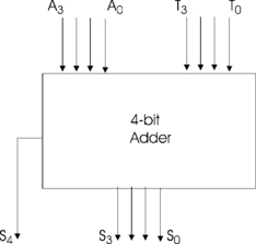
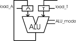
We wish to construct a circuit that will form the sum of two 4-bit numbers. Let these numbers be A = = <A3 A2 A1 A0> and T = = <T3 T2 T1 T0> while the sum of A and T is S = = <S4 S0 S2 S1 S0>.
The notation Yi refers to bit i of number Y. As noted in Chapter 1, the sum, S, has one more bit than A and T. Our aim is to make the device shown in Figure 4.1. This device has eight inputs and five outputs.
We could draw the truth table for this device and derive the logic expressions in a way similar to that used in Chapter 1. Since there are eight inputs, the truth table would have 28 (25 6) rows. However, if we want an adder to add two 8-bit numbers, there will be 16 inputs, giving 216 (65 536) rows! We will take another approach; we shall copy the way humans perform addition. Humans proceed by first adding A0 and T0 using the rules for adding two 1-bit numbers to produce a 2-bit sum:
We write down the right-hand bit of the 2-bit sum as part of the answer and carry the left-hand bit into the column to the left. Now when we add bits A1 and T1 we also add the carry from the previous column. We continue in this way until all the 4 bits in the numbers have been added. Using this method, the adder design becomes as shown in Figure 4.2, which shows how the 4-bit adder can be made from four identical 1-bit adders. The 1-bit adder is traditionally called a full adder.

We can easily design the circuit of the full adder using the truth-table method from Chapter 2. The truth table of the required logic is given in Figure 4.3. After simplification we obtain the expressions for the logic of the full adder:

Si = /Ci./Ai.Ti + /Ci.Ai./Ti + Ci./Ai./Ti + Ci.Ai.Ti
Connecting four of these devices as in Figure 4.2 results in the required 4-bit adder. This adder has a width of 4 bits; it can readily be extended to produce an adder of any width. This form of adder circuit is called a ripple carry adder, a name which indicates its main weakness; that C4 cannot be generated until C3 has been generated, but C3 cannot be generated until C2 has been generated, and so on. The ripple-carry adder is therefore quite slow. Later, we will investigate a faster circuit.
4.2 Adder/Subtractor
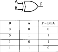
We can extend the adder to make it perform subtraction as well as addition. Recall from Chapter 1 that subtraction may be performed by ‘change the sign and add’. Changing the sign of a two’s complement number, or multiplying it by −1, simply requires inversion of all the bits and adding 1. The inversion can be implemented by using an exclusive-OR, XOR, gate. The truth table and symbol for this gate are shown in Figure 4.4. Note that if input B = = 1, the output is the complement of A while if B = = 0, the output is the same as A. Thus, we have a device that can be made to behave both like a NOT gate or a direct connection according to input signal B. We place these gates at one of the inputs to an adder circuit, Figure 4.5. When control signal ALU_mode is set to 1, the XOR gates behave as inverters and the carry into the first stage of the adder is forced to 1. The output from the adder is thus A + (−T), or A – T. When control signal ALU_mode is set to 0, the XOR gates behave as direct connections and the carry into the adder is forced to 0, so that the output is A plus B. We now have an adder/subtractor circuit whose function is determined by the control signal, ALU_mode.

4.3 Arithmetic and logic unit
As well as addition and subtraction, a programmer is likely to want to perform logical operations such as AND and OR. We can include these functions in a variety of ways. The most straightforward way to incorporate these functions is to include an AND gate and an OR gate into the circuit and use a multiplexer to select the required output signal, Figure 4.6. Because the device can now perform four functions, it requires two1 control signals, ALU_mode0 and ALU_mode1, in order to select a particular function. These signals are connected to the select inputs of the multiplexer, and ALU_mode0 is also connected to C0, the carry-in of the first stage of the complete circuit. You should verify that when the ALU_mode signals are set to the values shown in the function table, the indicated functions are performed. Since the device performs arithmetic as well as logical operations, it is called an arithmetic and logic unit, or ALU.
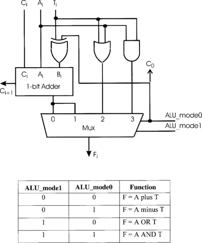
Figure 4.7 shows an 8-bit ALU together with its associated registers, A and T. The registers hold 8 bits and the broad lines represent eight individual wires, one for each bit. Since the registers are edge triggered flip-flops, when control signal load_T changes from low to high it causes the data present at the input of register T to be stored in the register. Similarly, a rising edge on load_A loads register A with the number at the output of the ALU. The inputs to the ALU are thus the numbers stored in registers A and T. For example, to add a number, num2, to the number num1, which is currently in register A, we must perform the sequence of operations in Figure 4.8.

We shall see the ALU in operation when we execute programs on the G80. For example, we shall see that in order to perform an instruction to subtract the number stored in register T from the number currently stored in the accumulator, the control unit sets the ALU_mode signals to the pattern that makes the ALU into a subtractor. After a very short delay (even electricity takes time to flow!), the output of the ALU becomes the current contents of the accumulator minus the contents of register T. This number is then loaded into the accumulator, replacing the original contents.
The ALU developed in this chapter does not provide for multiplication and division. We shall perform these operations in software; these programs will require that data can be shifted, an operation that we consider next.
4.4 Shifting data
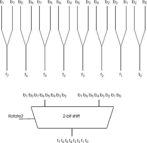
It is often convenient to be able to shift a pattern of bits to the left or right. More generally, we may wish to shift circularly or rotate data. In this type of shift, the bits that reach the end of the bit pattern when shifted are fed into the other end. Thus, the bits, <b7 b6 b5 b4 b3 b2 b1 b0>, when rotated 2 bits to the right, become <b1 b0 b7 b6 b5 b4 b3 b2>. This could be achieved by placing the data into a shift register and generating two shift pulses. Rotations to the left might be achieved by making the shift register bi-directional, or by obtaining an N-bit rotate to the left by rotating right 8-N places. However, this implementation will be very slow, particularly if the data were, say, 32 bits and a rotation by many bits is required. We seek a faster way of rotating data.
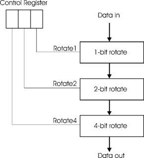
Eight two-way multiplexers, Figure 4.9, are connected so that they rotate the data right 2 bits. The multiplexer control signal is labelled Rotate2 since, when it is asserted, the device rotates the data two places while if not asserted the data passes through the device unchanged. We can make similar circuits that rotate one place and four places. When these are connected as shown in Figure 4.10, we have a device that is called a barrel shifter. The control register holds the number of places to rotate. For example, if this register is loaded with the number 5, the 4-bit shifter and the 1-bit shifter will actually shift the data while the 2-bit shifter passes its input unchanged to its output. The output data is thus rotated by the required 5 bits.
4.4 Fast adders*
A great deal of effort has gone into the design of ALU circuits that operate faster than those based on the ripple carry adder. We have noted earlier that the ripple carry adder is slow because each adder stage can form its outputs only when all the earlier stages have produced theirs2. Since stage i produces a carry-out bit, Ci+1, that depends on the inputs Ai, Ti, and Ci, it is possible to obtain logic equations for the carry-out from each stage.
Our first attempt is to use the relationship derived earlier:
= A1.T1 + A1.(A0.T0 + A0.C0 + T0.C0) + T1.(A0.T0 + A0.C0 + T0.C0)
= A1.T1 + A1.A0.T0 + A1.A0.C0 + A1.T0.C0 + T1.A0.T0 + T1.A0.C0 + T1.T0.C0
Similarly, we can write expressions for C3, C4, and so on. Theoretically, these expressions allow us to design a logic circuit to produce all the carry signals at the same time using two layers of gates. Unfortunately, the expressions become extremely long; give a thought to how the expression for C31 would look! We do not pursue this possible solution any further because the number of gates becomes extremely large.
Our second attempt at a solution will result in a practical fast adder. The so-called carry-look-ahead3 ALU generates all the carry signals at the same time, although not as quickly as our first attempt would have done. Reconsider the truth table for the adder, Figure 4.3. Note that when Ai and Ti have different values, the carry-out from the adder stage is the same as the carry-in. That is, when Ai./Ti + /Ai.TI = = 1, then Ci+1 = Ci; we regard this as the carry-in ‘propagating’ to the carry-out. Also, when Ai and Ti are both 1, Ci+1 = 1, that is, when Ai.Ti = = 1, then Ci+1 = 1; we regard this as the carry-out being ‘generated’ by the adder stage. Putting these expressions together, we have:
Ci+1 = (Ai./Ti + /Ai.Ti).Ci + Ai.Ti.
For brevity, let Pi = Ai + Ti and let Gi = Ai.Ti.
This is really a formal statement of common sense. The carry-out, Ci+1, is 1 if the carry-in, Ci, is a 1 AND the stage propagates the carry through the stage OR if the carry-out is set to 1 by the adder stage itself. At first sight, this does not appear to be an improvement over the ripple-carry adder. However, we persevere with the analysis; putting i = 0, 1, 2, 3, …, we obtain:

We can readily make a 4-bit adder from these equations. However, the equations are becoming rather large, implying that a large number of gates will be required to produce C31. To overcome this difficulty, let us regard a 4-bit adder as a building block, and use four of them to make a 16-bit adder. We could simply connect the carry-out of each 4-bit adder to the carry-in of the next 4-bit adder, as shown in Figure 4.11(a). In this case, we are using a ripple-carry between the 4-bit blocks. Alternatively, we can regard each 4-bit block as either generating or propagating a carry, just as we did for the 1-bit adders. This allows us to devise carry-look-ahead logic for the carry-in signals to each 4-bit adder block, as shown in Figure 4.11(b). (The logic equations turn out to be the same as that for the 1-bit adders.) We now have a 16-bit adder made from four blocks of 4-bit adders with carry-look-ahead logic. Wider adders can be made by regarding the 16-bit adder as a building block and, again, similar logic allows us to produce carry-look-ahead circuits for groups of 16-bit adders. Even though there are now several layers of look-ahead logic, this adder has a substantial advantage in speed of operation when compared with the ripple-carry-adder. As is often the case, this speed advantage is at the expense of a more complex circuit.

4.5 Floating-point numbers*
An 8-bit number allows us to represent unsigned integers in the range 0 to 28–1 (255). If we choose to regard the bits as a signed integer, the range becomes −27 (−128) to +27–1 (+127). In either case, there are 256 different numbers. Numbers with 16 bits extend these ranges to 0 to 216–1 (65 535) and −215 (−32 768) to +215–1 (+32 767); in both cases 216 different numbers are represented. If we wish to use larger integers, we simply use more bits in the number. For example, using 32-bit numbers gives us 232 (approximately 4 000 000 000) different numbers, which we can regard as unsigned integers in the range 0 to 232–1 and signed integers −231 to + 231 −1. Whatever the number of bits, these integer numbers effectively have the binary point at the right-hand end of the number. If we regard the binary point as being two places from the right-hand end, we have a binary fraction. Thus, the 8-bit number 000101.11 has the decimal value 5.75, since the bits after the binary point have weights of 2–1 (0.5) and 2–2 (0.25). All these numbers are called fixed point numbers, because the binary point is always at the same, fixed, position in every number.
Suppose we wish to cope with very large and very small numbers, such as the decimal numbers 5 432 678 123 456 and 0.000 000 000 000 432 196. If the sum of these two numbers must be exactly 5 432 678 123 456.000 000 000 000 432 196, a number must be represented by a very large number of bits. Usually this amount of precision is not required and some approximation of the number is acceptable. In such cases, we can use floating-point numbers.
The decimal number 5 432 678 123 456 may be represented in floating-point format as 5.432 678 123 456 × 1012 and 0.000 000 000 000 432 196 as 4.32 196 × 10–13. This number representation actually uses two numbers, the mantissa4, and the exponent. Thus, 4.32 196 × 10–13 has a mantissa of 4.32 196 and an exponent of −13, so may be represented by the two numbers 4.32 196 and −13.
Clearly, we may choose to store the mantissa and exponent in any number of bits. Manufacturers of early computers used different ways of representing these numbers, which caused difficulties when transferring programs and data between different computers. A committee of the IEEE5 agreed a standard for floating-point numbers in 1985, called IEEE standard 754 (1985). We will adhere to this standard in our discussion.
For binary numbers, we may write:
The floating-point representations of these numbers are written in the form 1.xxxx × 2E, that is the first bit of the number is always 1. This is called the normalized representation. Since the first bit of a normalized number is always 1, there is no need to store it. Thus, number 1.bb..bbbb × 2E will be stored as the two quantities F and E, where F = 0.bb..bbbb, it being assumed that the first bit of F is 1. We now have: number = (1 + F) × 2E.
To accommodate signed numbers, we add a sign bit, S, such that if S = = 0, the number is positive.
We now have: number = (−1)S × (1 + F) × 2E.
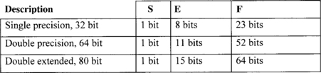
The IEEE 754 provides for floating-point numbers of various lengths; the most popular of these have the formats shown in Figure 4.12.
The exponent, E, is stored as a biased number, so that the 8-bit exponent of single precision numbers is written:
![]()
That is, E is biased by 127; the value of E is obtained by subtracting 127 from its pure binary value. Thus, number = (−1)S × (1 + F) × 2E–127. The 11-bit exponent used in double precision numbers is biased by 1023. This apparently strange representation simplifies the comparison of the exponents in two numbers during addition and subtraction of floating-point numbers.
4.5.1 Special quantities
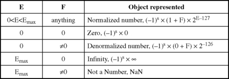
Let us look closely at the representation of zero. When we write the smallest magnitude by setting E = 0 and F = 0, the formula for single precision numbers gives (−1)0 × (1 + 0) × 20–127 =+ 1 × 2–127, which is very small, but not exactly zero. However, the IEEE 754 standard defines the all 0s number as zero. This is not only logically pleasing but it also facilitates checking to see if a number is zero, for example to prevent division by zero. The IEEE standard also defines the extreme values of E to signify infinity, and other objects, as shown in Figure 4.13. The table shows that the result of some arithmetic operations should return with E = 255 and F > 0, which indicates that it is not a number, NaN. For example, the result should be NaN after attempting to perform ∞ + ∞, ∞ – ∞, 0 × ∞, 0/0, and ∞/∞.
4.5.2 Smallest and largest numbers
What is the smallest number that can be represented in single precision? Since numbers may be positive or negative, we will concern ourselves only with the magnitude of the numbers.
Clearly, the smallest number is zero, which is defined as having E = 0, F = 0.
However, the smallest non-zero number has E = 1, F = 0, giving a magnitude of:
1.00000000000000000000000 × 21–127
The largest value for E is 254, since 255 is used to represent infinity or NaN. The largest value of F is 11111111111111111111111 (23 bits), so the number with the largest magnitude is:
1.11111111111111111111111 × 2254–127
If the result of floating-point arithmetic is a number larger than this, the number is said to overflow and the result should be set to E = 255, F > 0, which indicates that the result is not a number, NaN.
4.5.3 Denormalized numbers
Considering single precision numbers only, we have seen that the smallest non-zero number has a magnitude of 1.0 × 2–126. Tiny numbers, those between zero and 1.0 × 2–126 are too small to be represented as normalized numbers, which are evaluated according to the formula, (−1)S × (1 + F) × 2E–127. Instead, these tiny, denormalized, numbers are stored as E = 0, F > 0, but are evaluated by (−1)S × (0 + F) × 2–126, that is, a 1 is not added to F and the exponent is always −126.
The largest denormalized number is stored as:
E = 0 F= 11111111111111111111111 (23 bits) and evaluated as:
number = 0.11111111111111111111111 × 2–126
The smallest denormalized number is stored as:
E = 0F= 00000000000000000000001 (23 bits) and evaluated as:
number = 0.00000000000000000000001 × 2–126
If the result of floating-point arithmetic is a number smaller than this, the number is said to underflow and the result should be set to E = 255, F > 0, which indicates that the result is not a number, NaN. Since denormalized numbers may have leading 0s in them, their precision is less than that of normalized numbers.
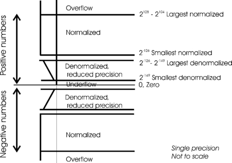
The whole number range is represented in Figure 4.14.
4.5.4 Multiplication and division
Floating-point multiplication and division are based on the rules:
Given X = a × 2p and Y = b × 2q,
The steps for multiplication are thus:
We shall use decimal numbers to illustrate these steps for multiplication and assume that the computer stores four decimal digits in the mantissa and two decimal digits in the exponent.
Step 1: Neither operand is zero, so continue.
Step 2: Add the exponents. 7 + (−4) = 3
(If the exponents are biased, we must subtract the bias.)
Step 3: Multiply the mantissae.

0.04670400 × 103 = 0.4670400 × 10²
(Check that exponent has not overflowed or underflowed.)
0.4670400 × 10² rounds to 0.4670 × 10²
If the operands have the same sign, the result is positive, otherwise it is negative. Here, the result is positive.
4.5.5 Addition and subtraction
Step 1: Neither operand is zero, so continue.
Step 2: Shift the smaller number until its exponent is the same as that of the larger number. 0.1321 101 = 0.001321 × 10³, which becomes 0.0013 × 10³ because the machine can hold only four digits.

Step 4: Normalize 1.0005 × 103 = 0.10005 × 10⁴.
4.5.6 Rounding
The IEEE standard requires that ‘all operations … shall be performed as if correct to infinite precision, then rounded’. If intermediate results are rounded to fit the number of bits available, then precision is lost. To meet this requirement, 2 additional bits, called guard and round, are saved at the right hand of the number.
The standard actually defines four rounding methods:
(i) Round towards zero – truncate
Simply ignore any extra bits. The rounded result is nearer to zero than the unrounded number.
The rounded result is nearer to + ∞ than the unrounded number.
The rounded result is nearer to – ∞ than the unrounded number.
This determines what to do if the number is at the halfway value. Instead of always rounding a number such as 0.72185 to 0.7219, this is done only half the time. For example, 3.25 rounds to 3.2 while 3.75 rounds to 3.8. Thus, the last digit is always even, which gives the method its name. For a large array of numbers, this method tends to ‘average out’ the error due to rounding.
In binary, if the bit in the least significant position (not including guard and round bits) is 1, add 1 in this position, else, truncate. This requires an extra bit, the sticky bit. This bit is set whenever there are non-zero bits to the right of the round bit. For example, in decimal, 0.500. 0001 will set the sticky bit. When the number is shifted to the right, so that the least significant digit gets lost, sticky indicates that the number is truly greater than 0.5 so the machine can round accordingly.
4.5.7 Precision
It should not be forgotten that there are only 232 different bit patterns in the 32-bit single precision representation of floating-point numbers so there are at most only 232 different floating-point numbers. Since there is an infinity of real numbers, a floating-point number can only approximate a real number. One result of this is that the addition of two numbers of very different magnitudes may result in the smaller number being effectively zero. Care must be exercised in the design of complicated numerical algorithms in order to preserve their accuracy. Consider the computation of x + y + z, where x = 1.5 × 1030, y =–1.5 × 1030, and z = 1.0 × 10⁻⁹ Computing (x + y) + z gives:

Thus, we have that (x + y) + z ≠ x + (y + z).
Large computers usually incorporate a hardware floating-point unit, FPU, which performs the arithmetic operations according to the IEE 754 standard. These FPUs also compute square roots and functions such as sin(), cos(), and log(). If we wish to use floating point in a small computer without an FPU, we shall have to write program code to perform the operations.
We can now design a computing machine using the concepts and digital devices we have considered.
4.6 Problems
1. Two methods of generating the carry-out from an adder stage were considered under the heading ‘Fast Adders’.
(i) The first method was said to be impractical because the length of the logical expression for Cn becomes extremely large for a large n. How many product terms are there in the expression for Cn? Assuming a 16-bit adder, how many product terms are there in the expression for C16?
(ii) The second method, carry-look-ahead, gives Cn in terms of P and G. How many product terms are there in the expression for Cn? How many product terms for C16?
2. What decimal number does the IEEE 32-bit standard number 11000000011000000000000000000000 represent?
3. Convert the decimal number + 10.75 to the IEEE 32-bit standard floating-point representation.
4. Convert +1.0 × 2125 to the IEEE 32-bit standard floating-point representation.
5. Convert +1.0 × 2–125 to the IEEE 32-bit standard floating-point representation.
6. It is required to evaluate the sum (+2125) + (+2–125), assuming IEEE 32-bit standard floating point representation. What will be the result?
1Remember that there are 2N different patterns of N binary signals.
2Charles Babbage recognized this problem and produced a mechanism for high speed carries for his decimal computer, in the 1830s.
3The carry-look-ahead solution described here was devised by O. L. MacSorley in 1961.
4The mantissa is sometimes called the significand.
5The IEEE is the Institution of Electrical and Electronic Engineers, based in the USA.