
3 Polynomial and Rational Functions

Chapter Outline
3.2 Division of Polynomial Functions
3.3 Zeros and Factors of Polynomial Functions
3.4 Real Zeros of Polynomial Functions
3.1 Polynomial Functions
![]() Introduction In Chapter 2 we graphed functions such as y = 3, y = 2x – 1, y = 5x2 – 2x = 4, and y = x3. These functions, in which the variable x is raised to a nonnegative integer power, are examples of a more general type of function called a polynomial function. Our goal in this section is to present some general guidelines for graphing such functions. First we state the formal definition of a polynomial function.
Introduction In Chapter 2 we graphed functions such as y = 3, y = 2x – 1, y = 5x2 – 2x = 4, and y = x3. These functions, in which the variable x is raised to a nonnegative integer power, are examples of a more general type of function called a polynomial function. Our goal in this section is to present some general guidelines for graphing such functions. First we state the formal definition of a polynomial function.
POLYNOMIAL FUNCTION
A polynomial function y = f(x) is a function of the form
![]()
where the coefficients an, an–1,…, a2, a1, a0 are real constants and n is a nonnegative integer.
The domain of any polynomial function f is the set of all real numbers (−∞, ∞).
The following functions are not polynomials:

The function
![]()
is a polynomial, where we interpret the number 4 as the coefficient of x0. Since 0 is a nonnegative integer, a constant function such as y = 3 is a polynomial function because it is the same as y = 3x0.
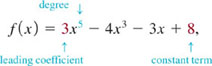
![]() Degree Polynomial functions are classified by their degree. The highest power of x in a polynomial is said to be its degree. So if an ≠ 0, then we say that f(x) in (1) has degree n. The number an in (1) is called the leading coefficient and a0 is called the constant term of the polynomial. For example,
Degree Polynomial functions are classified by their degree. The highest power of x in a polynomial is said to be its degree. So if an ≠ 0, then we say that f(x) in (1) has degree n. The number an in (1) is called the leading coefficient and a0 is called the constant term of the polynomial. For example,
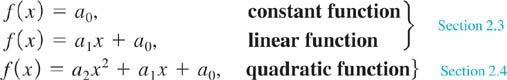
is a polynomial function of degree 5. We have already studied special polynomial functions in Sections 2.3 and 2.4. Polynomials of degrees n = 0, n = 1, and n = 2 are, respectively,
Polynomials of degrees n = 3,n = 4, and n = 5 are, in turn, commonly referred to as cubic, quartic, and quintic functions. The constant function f(x) = 0 is called the zero polynomial.
![]() Graphs Recall that the graph of a constant function f(x) = a0 is a horizontal line, the graph of a linear function f(x) = a1x + a0 is a line with slope m = a1, and the graph of a quadratic function f(x) = a2x2 + a1x + a0 is a parabola. See Sections 2.3 and 2.4. Such descriptive statements cannot be made about the graph of a higher-degree polynomial function. What is the shape of the graph of a fifth-degree polynomial function? It turns out that the graph of a polynomial function of degree n ≥ 3 can have several possible shapes. In general, graphing a polynomial function f of degree n ≥ 3 often demands the use of either calculus or a graphing utility. However, we will see in the discussion that follows that by determining
Graphs Recall that the graph of a constant function f(x) = a0 is a horizontal line, the graph of a linear function f(x) = a1x + a0 is a line with slope m = a1, and the graph of a quadratic function f(x) = a2x2 + a1x + a0 is a parabola. See Sections 2.3 and 2.4. Such descriptive statements cannot be made about the graph of a higher-degree polynomial function. What is the shape of the graph of a fifth-degree polynomial function? It turns out that the graph of a polynomial function of degree n ≥ 3 can have several possible shapes. In general, graphing a polynomial function f of degree n ≥ 3 often demands the use of either calculus or a graphing utility. However, we will see in the discussion that follows that by determining
- shifting,
- end behavior,
- symmetry,
- intercepts, and
- local behavior
of the function we can, in some instances, quickly sketch a reasonable graph of a higher-degree polynomial function while keeping point-plotting to a minimum. Before elaborating on each of these concepts we return to the notion of a power function first introduced in Section 2.2.
![]() Power Function A special case of the power function (see Section 2.2) is the single-term polynomial function or monomial,
Power Function A special case of the power function (see Section 2.2) is the single-term polynomial function or monomial,
![]()
The graphs of f for degrees n = 1, 2, 3, 4, 5, and 6 are given in FIGURE 3.1.1. The interesting fact about (2) is that all the graphs for n odd are basically the same. The notable characteristics are that the graphs are symmetric about the origin and become increasingly flatter near the origin as the degree n increases. See Figures 3.1.1(a)–3.1.1(c). A similar observation is true for the graphs of (2) for n even, except, of course, the graphs are symmetric with respect to the y-axis. See Figures 3.1.1(d)–3.1.1(f).
![]() Shifted Graphs Recall from Section 2.2 that for c > 0, the graphs of polynomial functions of the form
Shifted Graphs Recall from Section 2.2 that for c > 0, the graphs of polynomial functions of the form
![]()
can be obtained by vertical and horizontal shifts of the graph of y = axn. Also, if the leading coefficient a is positive, the graph of y = axn is either a vertical stretch or a vertical compression of the graph of the basic single-term polynomial function f(x) = xn. When a is negative we also carry out a reflection in the x-axis.
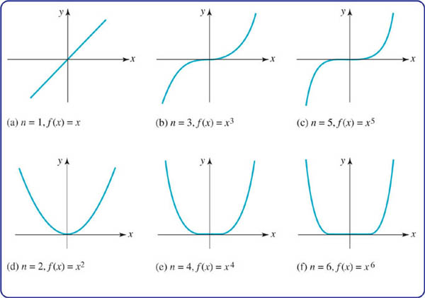
FIGURE 3.1.1 Brief catalogue of power functions f(x) = xn, n = 1, 2, …, 6
EXAMPLE 1 Graphing a Shifted Polynomial Function
The graph of y = −(x = 2)3 − 1 is the graph of f(x) = x3 reflected in the x-axis, shifted 2 units to the left, and then shifted vertically downward 1 unit. First review Figure 3.1.1(b) and then see FIGURE 3.1.2.
![]()
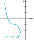
FIGURE 3.1.2 Reflected and shifted graph in Example 1
![]() End Behavior The knowledge of the shape of a single-term polynomial function f(x) = xn is important for another reason. First, examine the computer-generated graphs given in FIGURES 3.1.3 and 3.1.4. Although the graph in Figure 3.1.3 certainly resembles the graphs in Figures 3.1.1(b) and 3.1.1(c), and the graph in FIGURE 3.1.4 resembles the graphs in Figure 3.1.1(d)–(f), the functions graphed in these two figures are not power functions f(x) = xn, odd, or f(x) = xn, even. We will not tell you at this point what the specific functions are except to say that they were both graphed on the interval [ −1000, 1000]. The point is this: the function whose graph is given in Figure 3.1.3 could be almost any polynomial function
End Behavior The knowledge of the shape of a single-term polynomial function f(x) = xn is important for another reason. First, examine the computer-generated graphs given in FIGURES 3.1.3 and 3.1.4. Although the graph in Figure 3.1.3 certainly resembles the graphs in Figures 3.1.1(b) and 3.1.1(c), and the graph in FIGURE 3.1.4 resembles the graphs in Figure 3.1.1(d)–(f), the functions graphed in these two figures are not power functions f(x) = xn, odd, or f(x) = xn, even. We will not tell you at this point what the specific functions are except to say that they were both graphed on the interval [ −1000, 1000]. The point is this: the function whose graph is given in Figure 3.1.3 could be almost any polynomial function
![]()
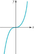
FIGURE 3.1.3 Mystery graph #1
an > 0, of odd degree n, n = 3, 5, … when graphed on [ − 1000, 1000]. Similarly, the graph in Figure 3.1.4 could be that of any polynomial function given in (1), with an > 0, of even degree n,n = 2,4, … when graphed on a large interval around the origin. As the next theorem indicates, the terms enclosed in the colored rectangle in (3) are irrelevant when we look at a graph of a polynomial globally—that is, for |x| large. How a polynomial function f behaves when |x| is very large is said to be its end behavior.
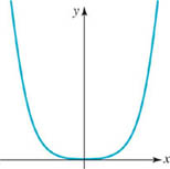
FIGURE 3.1.4 Mystery graph #2
END BEHAVIOR
For |x| very large, that is, for x → − ∞ and x → ∞, the graph of the polynomial function f(x) = anxn = an −1xn−1 = … = a2x2 = a1x = a0, resembles the graph of y = anxn.
To see why the graph of a polynomial function such as f(x) = −2x3 + 4x2 + 5 resembles the graph of the single-term polynomial y = −2x3 when |x| is large, let’s factor out the highest power of x, that is, x3:
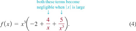
By letting |x| increase without bound, both 4/x and 5/x3 can be made as close to 0 as we want. Thus when |x| is large, the values of the function f in (4) are closely approximated by the values of y = −2x3.
There can be only four types of end behavior for a polynomial function f. Although two of the end behaviors are already illustrated in Figures 3.1.3 and 3.1.4, we include them again in the pictorial summary given in Figure 3.1.5. To interpret the arrows in FIGURE 3.1.5 let’s examine Figure 3.1.5(a). The position and direction of the left arrow (left arrow points down) indicates that as x → −∞, the values f(x) are negative and large in magnitude. Stated another way, the graph is heading downward as x → −∞. Similarly, the position and direction of the right arrow (right arrow points up) indicates that the graph is heading upward as x → ∞.
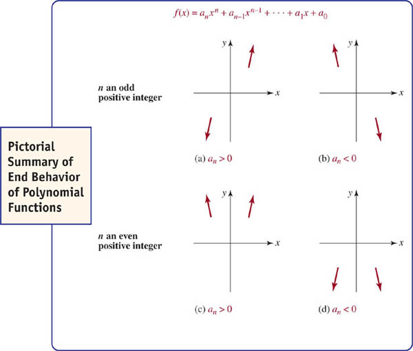
FIGURE 3.1.5 End behavior of a polynomial function f depends on its degree n and on the sign of its leading coefficient an
The gaps between the arrows in Figure 3.1.5 correspond to some interval around the origin. In these gaps the graph of f exhibits local behavior, in other words, the graph of f shows the characteristics of a polynomial function of a particular degree. This local behavior includes the x- and y-intercepts of the graph, the behavior of the graph at an x-intercept, the turning points of the graph, and observable symmetry of the graph (if any). A turning point is a point (c, f(c)) at which the graph of a polynomial function f changes direction, that is, the function f changes from increasing to decreasing or vice versa. The graph of a polynomial function of degree n can have up to n − 1 turning points. In calculus a turning point corresponds to a relative, or local, extremum of a function f. A relative extremum of f is classified as either a maximum or a minimum. If (c, f(c)) is a turning point, then in some interval containing c, then f(c) is either the largest (relative maximum) or smallest (relative minimum) function value. If f(c) is a relative maximum, then the graph of a polynomial function f must change from increasing immediately to the left of c to decreasing immediately to the right of c, whereas if f(c) is a relative minimum the function f changes from decreasing to increasing at c. These concepts will be illustrated in Example 2.
![]() Symmetry It is easy to tell by inspection those polynomial functions whose graphs possess symmetry with respect to either the y-axis or the origin. The words “even” and “odd” functions have special meaning for polynomial functions. Recall that an even function is one for which f(−x) = f(x) and an odd function is one for which f(−x) = −f(x). These two conditions hold for polynomial functions in which all the powers of x are even integers and odd integers, respectively. For example,
Symmetry It is easy to tell by inspection those polynomial functions whose graphs possess symmetry with respect to either the y-axis or the origin. The words “even” and “odd” functions have special meaning for polynomial functions. Recall that an even function is one for which f(−x) = f(x) and an odd function is one for which f(−x) = −f(x). These two conditions hold for polynomial functions in which all the powers of x are even integers and odd integers, respectively. For example,
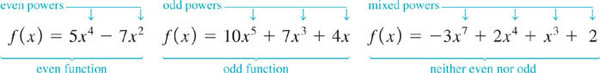
A function such as f(x) = 3x6 −x4 = 6 is an even function because the obvious powers are even integers; the constant term 6 is actually 6x0, and 0 is an even nonnegative integer.
![]() Intercepts The graph of every polynomial function f passes through the y-axis since x = 0 is the domain of the function. The y-intercept is the point (0, f(0)). Recall that a number c is a zero of a function f if f(c) = 0. In this discussion we assume c is a real zero. If x − c is a factor of a polynomial function f,that is, f(x) = (x − c)q(x) where q(x) is another polynomial, then clearly f(c) = 0 and the corresponding point on the graph is (c, 0). Thus the real zeros of a polynomial function are the x-coordinates of the x-intercepts of its graph. If (x − c)m is a factor of f, where m > 1 is a positive integer, and (x − c)m + 1 is not a factor of f, then c is said to be a repeated zero, or more precisely, a zero of multiplicity m. For example, f(x) = x2 − 10x + 25 is equivalent to f(x) = (x − 5)2. Hence 5 is a repeated zero or a zero of multiplicity 2. When m = 1, c is called a simple zero. For example,
Intercepts The graph of every polynomial function f passes through the y-axis since x = 0 is the domain of the function. The y-intercept is the point (0, f(0)). Recall that a number c is a zero of a function f if f(c) = 0. In this discussion we assume c is a real zero. If x − c is a factor of a polynomial function f,that is, f(x) = (x − c)q(x) where q(x) is another polynomial, then clearly f(c) = 0 and the corresponding point on the graph is (c, 0). Thus the real zeros of a polynomial function are the x-coordinates of the x-intercepts of its graph. If (x − c)m is a factor of f, where m > 1 is a positive integer, and (x − c)m + 1 is not a factor of f, then c is said to be a repeated zero, or more precisely, a zero of multiplicity m. For example, f(x) = x2 − 10x + 25 is equivalent to f(x) = (x − 5)2. Hence 5 is a repeated zero or a zero of multiplicity 2. When m = 1, c is called a simple zero. For example, ![]() are simple zeros of f(x) = 6x2 −x − 1 since f can be written as
are simple zeros of f(x) = 6x2 −x − 1 since f can be written as ![]() . The behavior of the graph of f at an x-intercept (c, 0) depends on whether c is a simple zero or a zero of multiplicity m > 1, where m is either an even or an odd integer.
. The behavior of the graph of f at an x-intercept (c, 0) depends on whether c is a simple zero or a zero of multiplicity m > 1, where m is either an even or an odd integer.
• If c is a simple zero, then the graph of f passes directly through the x-axis at (c, 0). See FIGURE 3.1.6(a).
• If c is a zero of odd multiplicity m = 3, 5,…, then the graph of f passes through the x-axis but is flattened at (c, 0). See Figure 3.1.6(b).
• If c is a zero of even multiplicity m = 2, 4,…, then the graph of f is tangent to, or touches, the x-axis at (c, 0). See Figure 3.1.6(c).
In the case when c is either a simple zero or a zero of odd multiplicity m = 3, 5,…, f(x) changes sign at (c, 0), whereas if c is a zero of even multiplicity m = 2, 4,…, f(x) does not change sign at (c, 0). We note that depending on the sign of the leading coefficient of the polynomial, the graphs in Figure 3.1.6 could be reflected in the x-axis. For example, at a zero of even multiplicity the graph of f could be tangent to the x-axis from below that axis.
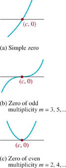
FIGURE 3.1.6 x-intercepts of a polynomial function f(x)
EXAMPLE 2 Graphing a Polynomial Function
Graph f(x) = x3 − 9x.
Solution Here are some of the things we look at to sketch the graph of f:
End Behavior: By ignoring all terms but the first, we see that the graph of f resembles the graph of y = x3 for large |x|. That is, the graph goes down to the left as x → −∞ and up to the right as x → ∞, as illustrated in Figure 3.1.5(a).
Symmetry: Since all the powers are odd integers, f is an odd function. The graph of f is symmetric with respect to the origin.
Intercepts: f(0) = 0, and so the y-intercept is (0, 0). Setting f(x) = 0,we see that we must solve x3 − 9x = 0. Factoring
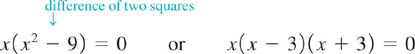
shows that the zeros of f are x = 0 and x = ± 3. The x-intercepts are (0, 0), (−3, 0), and (3, 0).
The Graph: From left to right, the graph rises (f is increasing) from the third quadrant and passes straight through (−3, 0) since −3 is a simple zero. Although the graph is rising as it passes through this intercept it must turn back downward (f decreasing) at some point in the second quadrant to get through the intercept (0, 0). Since the graph is symmetric with respect to the origin, its behavior is just the opposite in the first and fourth quadrants. See FIGURE 3.1.7.
![]()
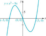
FIGURE 3.1.7 Graph of function in Example 2
In Example 2, the graph of f has two turning points. On the interval [ − 3, 0] there is a relative maximum of f and on the interval [0, 3] there is a relative minimum of f. We made no attempt to locate the turning points precisely; this is something that would, in general, require techniques from calculus. The best we can do using precalculus mathematics to refine the graph is to resort to plotting additional points on the intervals of interest. By the way, f(x) = x3 − 9x is the function whose graph on the interval [ −1000, 1000] is given in Figure 3.1.3.
EXAMPLE 3 Graphing a Polynomial Function
Graph f(x) = (1 −x)(x = 1)2.
Solution Multiplying out, f is the same as f(x) = −x3 −x2 = x = 1.
End Behavior: From the preceding line we see that the graph of f resembles the graph of y = −x3 for large |x|, just the opposite of the end behavior of the function in Example 2. See Figure 3.1.5(b).
Symmetry: As we see from f(x) = −x3 −x2 + x + 1, there are both even and odd powers of x present. Hence f is neither even nor odd; its graph possesses no y-axis or origin symmetry.
Intercepts: f(0) = 1 so the y-intercept is (0, 1). From the given factored form of f(x), we see that (− 1, 0) and (1, 0) are the x-intercepts.
The Graph: From left to right, the graph falls (f decreasing) from the second quadrant and then, because − 1 is a zero of multiplicity 2, the graph is tangent to the x-axis at (− 1, 0). The graph then rises (f increasing) as it passes through the y-intercept (0, 1). At some point within the interval [ − 1, 1] the graph turns downward (f decreasing) and, since 1 is a simple zero, passes through the x-axis at (1, 0), heading downward into the fourth quadrant. See FIGURE 3.1.8.
![]()
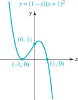
FIGURE 3.1.8 Graph of function in Example 3
In Example 3, there are again two turning points. It should be clear that the point (− 1, 0) is a turning point (f changes from decreasing to increasing at −1) and f(−1) = 0 is a relative minimum of f. There is a turning point (f changes from increasing to decreasing at this point) on the interval [ − 1, 1 ] and the function value at this point is a relative maximum of f.
EXAMPLE 4 Zeros of Multiplicity Two
Graph f(x) = x4 − 4x2 + 4.
Solution Before proceeding, note that the right-hand side of f is a perfect square. That is, f(x) = (x2 − 2)2. Since ![]() , by the laws of exponents we can write
, by the laws of exponents we can write
![]()
End Behavior: Inspection of f(x) shows that its graph resembles the graph of y = x4 for large |x|. That is, the graph goes up to the left as x → −∞ and up to the right as x → ∞, as shown in Figure 3.1.5(c).
Symmetry: Because f(x) contains only even powers of x, it is an even function and so its graph is symmetric with respect to the y-axis.
Intercepts: f(0) = 4, so the y-intercept is (0, 4). Inspection of (5) shows the x-intercepts are ![]() .
.
The Graph: From left to right, the graph falls from the second quadrant and then, because ![]() is a zero of multiplicity 2, the graph touches the x-axis at
is a zero of multiplicity 2, the graph touches the x-axis at ![]() . The graph then rises from this point to the y-intercept (0, 4).We then use the y-axis symmetry to finish the graph in the first quadrant. See FIGURE 3.1.9.
. The graph then rises from this point to the y-intercept (0, 4).We then use the y-axis symmetry to finish the graph in the first quadrant. See FIGURE 3.1.9.
![]()
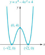
FIGURE 3.1.9 Graph of function in Example 4
In Example 4, the graph of f has three turning points. From the even multiplicity of the zeros, along with the y-axis symmetry, it can be deduced that the x-intercepts ![]() and
and ![]() are turning points and
are turning points and ![]() are relative minima, and that the y-intercept (0, 4) is a turning point and f(0) = 4 is a relative maximum.
are relative minima, and that the y-intercept (0, 4) is a turning point and f(0) = 4 is a relative maximum.
EXAMPLE 5 Zero of Multiplicity Three
Graph f(x) = − (x + 4)(x − 2)3.
Solution
End Behavior: Inspection of f shows that its graph resembles the graph of y = −x4 for large |x|. This end behavior of f is shown in Figure 3.1.5(d).
Symmetry: The function f is neither even nor odd. It is straightforward to show that f(−x) ≠ f(x) and f(−x) ≠ −f(x).
Intercepts: f(0) = (− 4)(−2)3 + 32, so the y-intercept is (0, 32). From the factored form of f(x), we see that (−4, 0) and (2, 0) are the x-intercepts.
The Graph: From left to right, the graph rises from the third quadrant and then, because −4 is a simple zero, the graph of f passes directly through the x-axis at (−4, 0). Somewhere within the interval [ −4, 0] the function f must change from increasing to decreasing to enable its graph to pass through the y-intercept (0, 32). After its graph passes through the y-intercept, the function f continues to decrease but, since 2 is a zero of multiplicity 3, its graph flattens as it passes through (2, 0), heading downward into the fourth quadrant. See FIGURE 3.1.10.
![]()
Note in Example 5 that since f is of degree 4, its graph could have up to three turning points. But as can be seen from Figure 3.1.10, the graph of f possesses only one turning point and at this point the function value is a relative maximum.
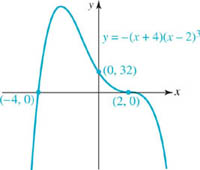
FIGURE 3.1.10 Graph of function in Example 5
EXAMPLE 6 Zeros of Multiplicity Two and Three
Graph f(x) 5 (x − 3)(x − 1)2(x + 2)3.
Solution The function f is of degree 6 and so its end behavior resembles the graph of y = x6for large |x|. See Figure 3.1.5(c). Also, the function f is neither even or odd; its graph possesses no y-axis or origin symmetry. The y-interceptis(0, f(0)) = (0, −24). From the factors of f we see that x-intercepts of the graph are (−2, 0), (1, 0), and (3, 0). Since −2 is a zero of multiplicity 3, the graph of f is flattened as it passes through (−2, 0). Since 1 is a zero of multiplicity 2, the graph of f is tangent to the x-axis at (1, 0). Since 3 is a simple zero, the graph of f passes directly through the x-axis at (3, 0). Putting all these facts together we obtain the graph in FIGURE 3.1.11.
![]()
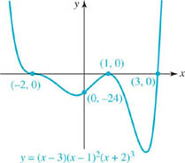
FIGURE 3.1.11 Graph of function in Example 6
In Example 6, since the function f is of degree 6 its graph could have up to five turning points. But as the graph in Figure 3.1.11 shows, there are only three turning points. At two of these points the unknown function values are relative minima; at the remaining point (1, 0), the function value f(1) = 0 is a relative maximum.
![]() Intermediate Value Theorem A polynomial function f is a continuous function. Recall that this means that the graph of y = f(x) has no breaks, gaps, or holes in it. The following result is a direct consequence of continuity.
Intermediate Value Theorem A polynomial function f is a continuous function. Recall that this means that the graph of y = f(x) has no breaks, gaps, or holes in it. The following result is a direct consequence of continuity.
INERMEDIATE VALUE THEOREM
Suppose y = f(x) is a continuous function on the closed interval [a, b]. If f(a) ≠ f(b) for a b,and if N is any number between f(a) and f(b), then there exists a number c in the open interval (a, b) for which f(c) = N.
As we see in FIGURE 3.1.12, the Intermediate Value Theorem simply states that f(x) takes on all values between the numbers f(a) and f(b). In particular, if the function values f(a) and f(b) have opposite signs, then by identifying N = 0, we can say that there is at least one number in (a, b) for which f(c) = 0. In other words, if either f(a) > 0, f(b) or f(a) 0, f(b) > 0, then f(x) has at least one zero c in the interval (a, b). The plausibility of this conclusion is illustrated in FIGURE 3.1.13.
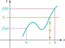
FIGURE 3.1.12 f(x) takes on all values between f(a) and f(b)
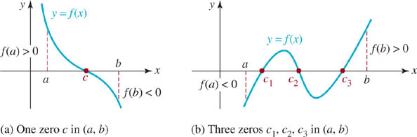
FIGURE 3.1.13 Locating zeros using the Intermediate Value Theorem
EXAMPLE 7 Using the Intermediate Value Theorem
Consider the function f(x) = x3 + x − 1. Since f is continuous on the interval [ −1, 1],
![]()
and 0 satisfies −3 < 0 < 1, we know from the Intermediate Value Theorem that the graph of f must cross the line y = 0 (the x-axis). More precisely, there is a real number c in the open interval (−1, 1) such that f(c) =0.
![]()
3.1 Exercises
Answers to selected odd-numbered problems begin on page ANS–9.
In Problems 1–8, proceed as in Example 1 and use transformations to sketch the graph of the given polynomial function.
1. y = x3 − 3
2. y = − (x + 2)3
3. y = (x − 2)3 + 2
4. y = 3 − (x + 2)3
5. y = (x − 5)4
6. y = x4 − 1
7. y = 1 (x − 1)4
8. y = 4 + (x + 1)4
In Problems 9–12, determine whether the given polynomial function f is even, odd, or neither even nor odd. Do not graph.
9. f(x) = − 2x3 + 4x
10. f(x) = x6 − 5x2 + 7
11. f(x) = x5 + 4x3 + 9x + 1
12. f(x) = x3(x + 2)(x − 2)
In Problems 13–18, match the given graph with one of the polynomial functions in (a) – (f).
(a) f(x) = x2(x − 1)2
(b) f(x) = −x3(x − 1)
(c) f(x) = x3(x − 1)3
(d) f(x) = −x(x − 1)3
(e) f(x) = −x2(x − 1)
(f) f(x) = x3(x − 1)2
13. 
FIGURE 3.1.14 Graph for Problem 13
14. 
FIGURE 3.1.15 Graph for Problem 14
15. 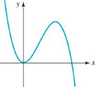
FIGURE 3.1.16 Graph for Problem 15
16. 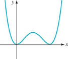
FIGURE 3.1.17 Graph for Problem 16
17. 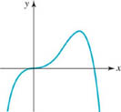
FIGURE 3.1.18 Graph for Problem 17
18. 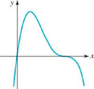
FIGURE 3.1.19 Graph for Problem 18
In Problems 19–22, construct a polynomial function f that has the given properties. There is no unique answer.
19. f is of degree 4, its graph is symmetric with respect to the y-axis, y-intercept is (0, − 6)
20. f is of degree 5, 0 is a zero of multiplicity 3, its graph is symmetric with respect to the origin
21. f has four real zeros, 1 is a simple zero, −3 is zero of multiplicity 2, behaves like y = − 7x4 for large values of |x|
22. f is of degree 6, has four real zeros, 2 is a zero of multiplicity 3, behaves like y = 2x6 for large values of |x|, f (0) = 8
In Problems 23–44, proceed as in Example 2 and sketch the graph of the given polynomial function f.
23. f(x) = x3 − 4x
24. f(x) = 9x −x3
25. f(x) = −x3 + x2 + 6x
26. f(x) = x3 + 7x2 + 12x
27. f(x) = (x + 1)(x − 2)(x − 4)
28. f(x) = (2 −x)(x + 2)(x + 1)
29. f(x) = x4 − 4x3 + 3x2
30. f(x) = x2(x − 2)2
31. f(x) = (x2 −x)(x2 − 5x + 6)
32. f(x) = x2(x2 + 3x + 2)
33. f(x) = (x2 − 1)(x2 + 9)
34. f(x) = x4 + 5x2 − 6
35. f(x) = −x4 + 2x2 − 1
36. f(x) = x4 − 6x2 + 9
37. f(x) = x4 + 3x3
38. f(x) = x(x − 2)3
39. f(x) = x5 − 4x3
40. f(x) = (x − 2)5 − 1x − 2)3
41. f(x) = 3x(x + 1)2(x − 1)2
42. f(x) = (x + 1)2(x − 1)3
43. ![]()
44. f(x) = x(x + 1)2(x − 2)(x − 3)
45. The graph of f(x) = x3 − 3x is given in FIGURE 3.1.20.
(a) Use the figure to obtain the graph of g(x) = f(x) + 2.
(b) Using only the graph obtained in part (a) write an equation, in factored form, for g(x). Then verify by multiplying out the factors that your equation for g(x) is the same as f(x) = 2 + x3 − 3x + 2.
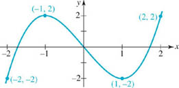
FIGURE 3.1.20 Graph for Problem 45
46. Find a polynomial function f of lowest possible degree whose graph is consistent with the graph given in FIGURE 3.1.21.
47. Find the value of k such that (2, 0) is an x-intercept for the graph of f(x) = kx5 −x2 + 5x + 8.
48. Find the values of k1 and k2 such that (− 1, 0) and (1, 0) are x-intercepts for the graph of f(x) = k1x4 − k2x3 + x − 4.
49. Find the value of k such that (0, 10)is the y-intercept for the graph of f(x) = x3 − 2x2 + 14x − 3k.
50. Consider the polynomial function f(x) = 1x − 2)n + 1(x + 5), where n is a positive integer. For what values of n does the graph of f touch, but not cross, the x-axis at (2, 0)?
51. Consider the polynomial function f(x) = (x − 1)n + 2(x + 1), where n is a positive integer. For what values of n does the graph of f cross the x-axis at (1, 0)?
52. Consider the polynomial function f(x) = (x − 5)2m(x + 1)2n−1, where m and n are positive integers.
(a) For what values of m does the graph of f cross the x-axis at (5, 0)?
(b) For what values of n does the graph of f cross the x-axis at (−1, 0) ?
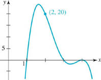
FIGURE 3.1.21 Graph for Problem 46
In Problems 53 and 54, use the Intermediate Value Theorem to determine whether there is a zero of the given function f in the indicated intervals. Do not graph.
53. f(x) = 60x3 − 13x2 − 145x − 28; [−2, −1], [−1, 0], [0, 1], [1, 2]
54. f(x) = 8x4 − 23x3 + 23x2 − 26x + 15; [−1, 0], [0, 1], [1, 2], [2, 3]
Miscellaneous Calculus-Related Problems
55. Constructing a Box An open box can be made from a rectangular piece of cardboard by cutting a square of length x from each corner and bending up the sides. See FIGURE 3.1.22. If the cardboard measures 30 cm by 40 cm, show that the volume of the resulting box is given by
![]()
Sketch the graph of V (x) for x > 0. What is the domain of the function V?
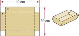
FIGURE 3.1.22 Box in Problem 55
56. Another Box In order to hold its shape, the box in Problem 55 will require tape or some other fastener at the corners. An open box that holds itself together can be made by cutting out a square of length x from each corner of a rectangular piece of cardboard, cutting on the solid line, and folding on the dashed lines, as shown in FIGURE 3.1.23. Find a polynomial function V(x) that gives the volume of the resulting box if the original cardboard measures 30 cm by 40 cm. Sketch the graph of V(x) for x > 0.
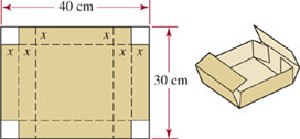
FIGURE 3.1.23 Box in Problem 56
57. Making a Cup A conical cup is made from a circular piece of paper of radius R by cutting out a circular sector and then joining the dashed edges as shown in FIGURE 3.1.24. Find a polynomial function V(h) that gives the volume of the conical cup in terms of its height.
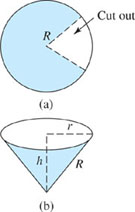
FIGURE 3.1.24 Cup in Problem 57
58. Hourglass Sand flows from the top half of the conical hourglass shown in FIGURE 3.1.25 to the bottom half at a constant rate. Find a polynomial function V(h) that gives the volume of the bottom pile of sand in terms of the height of the sand. Assume that the top of the pile is level. [Hint: Use similar triangles.]
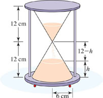
FIGURE 3.1.25 Hourglass in Problem 58
For Discussion
59. Examine Figure 3.1.5. Then discuss whether there can exist cubic polynomial functions that have no real zeros.
60. Suppose a polynomial function f has three zeros, −3, 2, and 4, and has the end behavior that its graph goes down to the left as x → −∞ and down to the right as x → ∞. Discuss possible equations for f.
Calculator/Computer Problems
In Problems 61 and 62, use a graphing utility to examine the graph of the given polynomial function on the indicated intervals.
61. f(x) = − (x − 8)(x + 10)2; [− 15, 15], [− 100, 100], [− 1000, 1000]
62. f(x) = (x − 5)2(x + 5)2; [− 10, 10], [− 100, 100], [− 1000, 1000]
3.2 Division of Polynomial Functions
![]() Introduction If p > 0 and s > 0 are integers such that p ≥ s, then p/s is called an improper fraction. By dividing p by s, we obtain unique numbers q and r that satisfy
Introduction If p > 0 and s > 0 are integers such that p ≥ s, then p/s is called an improper fraction. By dividing p by s, we obtain unique numbers q and r that satisfy
![]()
where0 ≤ r s. The number p is called the dividend, s is the divisor, q is the quotient, and r is the remainder. For example, consider the improper fraction ![]() . Performing long division gives
. Performing long division gives
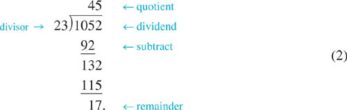
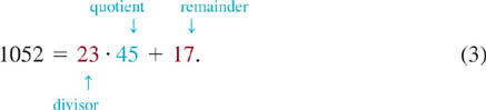
The result in (2) can be written as ![]() is a proper fraction since the numerator is less than the denominator; in other words, the fraction is less than 1. If we multiply this result by the divisor 23 we obtain the special way of writing the dividend p illustrated in the second equation in (1):
is a proper fraction since the numerator is less than the denominator; in other words, the fraction is less than 1. If we multiply this result by the divisor 23 we obtain the special way of writing the dividend p illustrated in the second equation in (1):
![]() Division of Polynomials The method for dividing two polynomial functions f(x) and d(x) is similar to division of positive integers. If the degree of a polynomial f(x) is greater than or equal to the degree of the polynomial d(x), then f(x)/d(x) is also called an improper fraction. A result analogous to (1) is called the Division Algorithm for polynomials.
Division of Polynomials The method for dividing two polynomial functions f(x) and d(x) is similar to division of positive integers. If the degree of a polynomial f(x) is greater than or equal to the degree of the polynomial d(x), then f(x)/d(x) is also called an improper fraction. A result analogous to (1) is called the Division Algorithm for polynomials.
DIVISION ALGORITM
Let f(x) and d(x) ≠ 0 be polynomials where the degree of f(x) is greater than or equal to the degree of d(x). Then there exist unique polynomials q(x) and r(x) such that

where r (x) has degree less than the degree of d(x).
The polynomial f(x) is called the dividend, d(x) the divisor, q(x) the quotient, and r(x) the remainder. Because r(x) has degree less than the degree of d(x), the rational expression r(x)/d(x) is called a proper fraction.
Observe in (4) when r(x) = 0, then f(x) = d(x)q(x), and so the divisor d(x) is a factor of f(x). In this case, we say that f(x) is divisible by d(x) or, in older terminology, d(x) divides evenly into f(x).
EXAMPLE 1 Division of Two Polynomials
Use long division to find the quotient q(x) and remainder r(x) when the polynomial f(x) = 3x3 −x2 − 2x + 6 is divided by the polynomial d(x) = x2 + 1.
Solution By long division,
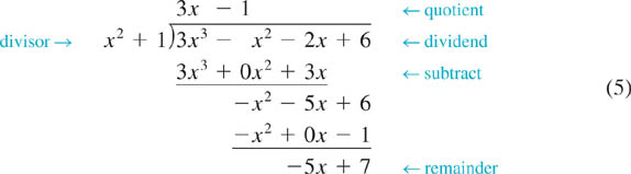
The result of the division in (5) can be written
![]()
If we multiply both sides of the last equation by the divisor x2 + 1, we get the second form given in (4):
![]()
![]()
If the divisor d(x) is a linear polynomial x − c, it follows from the Division Algorithm that the degree of the remainder r is 0, that is to say, r is a constant. Thus (4) becomes
![]()
When the number x = c is substituted into (7), we discover an alternative way of evaluating a polynomial function:
![]()
The foregoing result is called the Remainder Theorem.
REMAINDER THEOREM
If a polynomial f (x) is divided by a linear polynomial x = c, then the remainder r is the value of f(x) at x = c, that is, f(c) = r.
EXAMPLE 2 Finding the Remainder
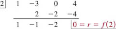
Use the Remainder Theorem to find r when f(x) = 4x3 − x2 = 4 is divided by x − 2.
Solution From the Remainder Theorem, the remainder r is the value of the function f evaluated at x = 2:
![]()
![]()
Example 2, where a remainder r is determined by calculating a function value f(c), is more interesting than important. What is important is the reverse problem: determine the function value f(c) by finding the remainder r by division of f by x − c. The next two examples illustrate this concept.
EXAMPLE 3 Evaluation by Division
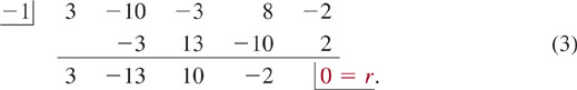
Use the Remainder Theorem to find f(c) for f(x) = x5 − 4x3 = 2x − 10 when c = −3.
Solution The value f(−3) is the remainder when f(x) = x5 − 4x3 + 2x − 10 is divided by x − (−3) + x + 3. For the purposes of long division we must account for the missing x4 and x2 terms by rewriting the dividend as
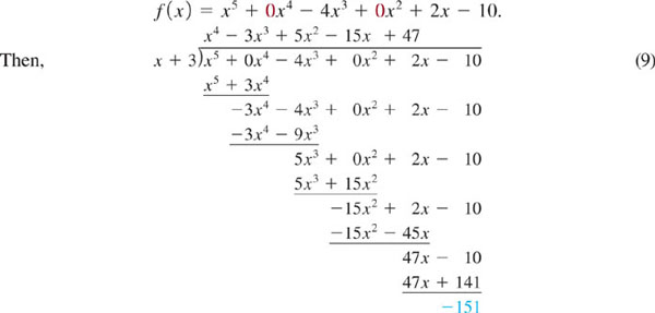
The remainder r in the division is the value of the function f at x = −3, that is, f(−3) = −151.
![]()
![]() Synthetic Division AfterworkingthroughExample3onecouldjustifiablyaskthe question: Why would anyone want to calculate the value of a polynomial function f by division? The answer is: We would not bother do this were it not for synthetic division. Synthetic division is a shorthand method of dividing a polynomial f(x) by a linear polynomial x − c; it does not require writing down the various powers of the variable x but only the coefficients of these powers in the dividend f(x) (which must include all 0 coefficients). It is also a very efficient and quick way of evaluating f(c), since the process utilizes only the arithmetic operations of multiplication and addition. No exponentiations such as 23 and 22 in (8) are involved. Here is the same division in (9) done synthetically:
Synthetic Division AfterworkingthroughExample3onecouldjustifiablyaskthe question: Why would anyone want to calculate the value of a polynomial function f by division? The answer is: We would not bother do this were it not for synthetic division. Synthetic division is a shorthand method of dividing a polynomial f(x) by a linear polynomial x − c; it does not require writing down the various powers of the variable x but only the coefficients of these powers in the dividend f(x) (which must include all 0 coefficients). It is also a very efficient and quick way of evaluating f(c), since the process utilizes only the arithmetic operations of multiplication and addition. No exponentiations such as 23 and 22 in (8) are involved. Here is the same division in (9) done synthetically:
![]() For a review of synthetic division please see the Student Resource Manual that accompanies this text.
For a review of synthetic division please see the Student Resource Manual that accompanies this text.
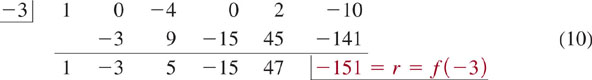
Recall that the bottom line of numbers in (10) are the coefficients of the various powers of x in the quotient q(x) when f(x) = x5 − 4x3 + 2x − 10 is divided by x + 3. You should compare this with the quotient obtained by the long division in (9).
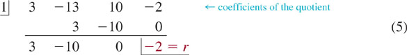
EXAMPLE 4 Using Synthetic Division to Evaluate a Function
Use the remainder theorem to find f(c) for
![]()
when c = 2.
Solution We will use synthetic division to find the remainder r in the division of f by x − 2. We begin by writing down all the coefficients in f(x), including 0 as the coefficient of x. From
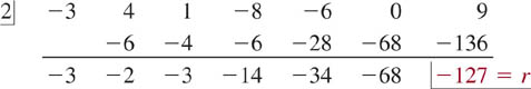
we see that f(2) = −127.
![]()
EXAMPLE 5 Using Synthetic Division to Evaluate a Function
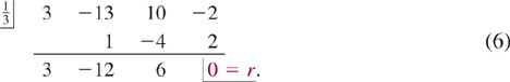
Use synthetic division to evaluate f(x) = x3 − 7x2 + 13x − 15 at x = 5.
Solution From the synthetic division
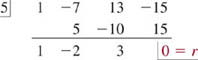
we see that f(5) = 0.
![]()
The result in Example 5 that f(5) = 0 shows that 5 is a zero of the given function f. Moreover, we have found additionally that f is divisible by the linear polynomial x − 5, or put another way, x − 5 is a factor of f. The synthetic division shows that f(x) = x3 − 7x2 + 13x − 15 is equivalent to
![]()
In the next section we will further explore the use of the Division Algorithm and the Remainder Theorem as a help in finding zeros and factors of a polynomial function.
3.2 Exercises
Answers to selected odd-numbered problems begin on page ANS–10.
In Problems 1–10, use long division to find the quotient q(x) and remainder r (x) when the polynomial f(x) is divided by the given polynomial d(x). In each case write your answer in the form f(x) = d(x)q(x) + r(x).
1. f(x) = 8x2 + 4x − 7; d(x) + x2
2. f(x) = x2 + 2x − 3; d(x) + x2 + 1
3. f(x) = 5x3 − 7x2 + 4x + 1; d(x) + x2 + x − 1
4. f(x) = 14x3 − 12x2 + 6; d(x) + x2 − 1
5. f(x) = 2x3 + 4x2 − 3x + 5; d(x) + (x + 2)2
6. f(x) = x3 + x2 + x + 1; d(x) + (2x + 1)2
7. f(x) = 27x3 + x − 2; d(x) + 3x2 −x
8. f(x) = x4 + 8; d(x) + x3 + 2x − 1
9. f(x) = 6x5 + 4x4 + x3; d(x) + x3 − 2
10. f(x) = 5x6 −x5 + 10x4 + 3x2 − 2x + 4; d(x) + x2 + x − 1
In Problems 11–16, proceed as in Example 2 and use the Remainder Theorem to find r when f(x) is divided by the given linear polynomial.
11. f(x) = 2x2 − 4x + 6; x − 2
12. f(x) = 3x2 + 7x − 1; x + 3
13. ![]()
14. f(x) = 5x3 + x2 − 4x − 6; x + 1
15. f(x) = x4 −x3 + 2x2 + 3x − 5; x − 3
16. ![]()
In Problems 17–22, proceed as in Example 3 and use the Remainder Theorem to find f(c) for the given value of c.
17. f(x) = 4x2 − 10x + 6; c + 2
18. ![]()
19. f(x) = x3 + 3x2 + 6x + 6;c + −5
20. ![]()
21. ![]()
22. f(x) = 14x4 − 60x3 + 49x2 − 21x +19; c + 1
In Problems 23–32, use synthetic division to find the quotient q(x) and remainder r (x) when f(x) is divided by the given linear polynomial.
23. f(x) = 2x2 −x + 5; x − 2
24. ![]()
25. f(x) = x3 −x2 + 2; x + 3
26. f(x) = 4x3 − 3x2 + 2x + 4; x − 7
27. f(x) = x4 + 16; x − 2
28. f(x) = 4x4 + 3x3 −x2 − 5x − 6; x + 3
29. f(x) = x5 + 56x2 − 4; x + 4
30. f(x) = 2x6 + 3x3 − 4x2 − 1; x + 1
31. ![]()
32. f(x) = x8 − 38; x − 3
In Problems 33–38, use synthetic division and the Remainder Theorem to find f(c) for the given value of c.
33. f(x) = 4x2 − 2x + 9; c + −3
34. ![]()
35. f(x) = 14x4 − 60x3 + 49x2 − 21x +19; c + 1
36. f(x) = 3x5 + x2 − 16; c + −2
37. f(x) = 2x6 − 3x5 + x4 − 2x + 1; c + 4
38. f(x) = x7 − 3x5 + 2x3 −x + 10; c + 5
In Problems 39 and 40, use long division to find a value of k such that f(x) is divisible by d(x).
39. f(x) = x4 + x3 + 3x2 + kx − 4; d(x) + x2 − 1
40. f(x) = x5 − 3x4 + 7x3 + kx2 + 9x − 5; d(x) + x2 −x + 1
In Problems 41 and 42, use synthetic division to find a value of k such that f(x) is divisible by d(x).
41. f(x) = kx4 + 2x2 + 9k; d(x) + x − 1
42. f(x) = x3 + kx2 − 2kx + 4; d(x) + x + 2
43. Find a value of k such that the remainder in the division of f(x) = 3x2 − 4kx + 1 by d(x) = x + 3 is r = −20.
44. When f(x) = x2 − 3x − 1 is divided by x − c, the remainder is r = 3. Determine c.
3.3 Zeros and Factors of Polynomial Functions
![]() Introduction In Section 2.1 we saw that a zero of a function f is a number c for which f(c) = 0. A zero c of a function f can be a real or a complex number. Recall that a complex number is a number of the form
Introduction In Section 2.1 we saw that a zero of a function f is a number c for which f(c) = 0. A zero c of a function f can be a real or a complex number. Recall that a complex number is a number of the form
![]()
and a and b are real numbers. The number a is called the real part of z and b is called the imaginary part of z. The symbol i is called the imaginary unit and it is common practice to write it as ![]() . If z = a + bi is a complex number, then
. If z = a + bi is a complex number, then ![]() is called its conjugate. Thus the simple polynomial function f(x) = x2 + 1 has two complex zeros since the solutions of x2 + 1 = 0 are
is called its conjugate. Thus the simple polynomial function f(x) = x2 + 1 has two complex zeros since the solutions of x2 + 1 = 0 are ![]() , that is, i and −i.
, that is, i and −i.
In this section we explore the connection between the zeros of a polynomial function f, the operation of division, and the factors of f.
![]() The arithmetic of complex numbers is reviewed in the Student Resource Manual.
The arithmetic of complex numbers is reviewed in the Student Resource Manual.
EXAMPLE 1 A Real Zero
Consider the polynomial function f(x) = 2x3 − 9x2 + 6x − 1. The real number ![]() is a zero of the function since
is a zero of the function since
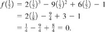
![]()
EXAMPLE 2 A Complex Zero
Consider the polynomial function f(x) = x3 − 5x2 + 8x − 6. The complex number 1 + i is a zero of the function. To verify this we use the binomial expansion of (a + b)3 and the fact that i2 = −1 and i3 = −i:
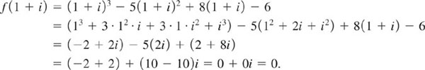
![]()
![]() Factor Theorem We can now relate the notion of a zero of a polynomial function f with division of polynomials. From the Remainder Theorem we know that when f(x) is divided by the linear polynomial x − c the remainder is r = f(c). If c is a zero of f, then f(c) = 0 implies r = 0. From the form of the Division Algorithm given in (4) of Section 3.2 we can then write f as
Factor Theorem We can now relate the notion of a zero of a polynomial function f with division of polynomials. From the Remainder Theorem we know that when f(x) is divided by the linear polynomial x − c the remainder is r = f(c). If c is a zero of f, then f(c) = 0 implies r = 0. From the form of the Division Algorithm given in (4) of Section 3.2 we can then write f as
![]()
Thus, if c is a zero of a polynomial function f, then x − c is a factor of f(x). Conversely, if x − c is a factor of f(x), then f has the form given in (1). In this case, we see immediately that f(c) = (c − c)q(c) = 0. These results are summarized in the Factor Theorem given next.
FACTOR THEOREM
A number c is a zero of a polynomial function f if and only if x − c is a factor of f(x).
Recall, if a polynomial function f is of degree n and (x − c)m, m ≤ n, is a factor of f(x), then c is said to be a zero of multiplicity m. When m = 1, c is a simple zero. Equivalently, we say that the number c is a root of multiplicity m of the equation f(x) = 0. We have already examined the graphical significance of repeated real zeros of a polynomial function f in Section 3.1. See Figure 3.1.6.
EXAMPLE 3 Factors of a Polynomial
Determine whether
(a) x = 1 is a factor of f(x) = x4 − 5x2 + 6x − 1,
(b) x − 2 is a factor of f(x) = x3 − 3x2 + 4.
Solution We use synthetic division to divide f(x) by the given linear term.
(a) From the division
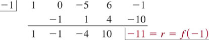
we see that f (−1) = −11 and so −1 is not a zero of f. We conclude that x − (−1) + x + 1 is not a factor of f(x).
(b) From the division
we see that f(2) = 0. This means that 2 is a zero and that x − 2 is a factor of f(x). From the division we see that the quotient is q(x) = x2 −x − 2 and so f(x) = (x − 2)(x2 −x − 2).
![]()
![]() Number of Zeros In Example 6 of Section 3.1 we graphed the polynomial function
Number of Zeros In Example 6 of Section 3.1 we graphed the polynomial function
![]()
The number 3 is a simple zero of f; the number 1 is a zero of multiplicity 2; and −2 is a zero of multiplicity 3. Although the function f has three distinct zeros (different from one another), it is, nevertheless, standard practice to say that f has six zeros because we count the multiplicities of each zero. Hence for the function f in (2), the number of zeros is 1 + 2 + 3 = 6. The question How many zeros does a polynomial function f have? is answered next.
FUNDAMENTAL THEOREM OF ALEGBRA
A polynomial function f of degree n > 0 has at least one zero.
The foregoing theorem, first proved by the German mathematician Carl Friedrich Gauss (1777–1855) in 1799, is considered one of the major milestones in the history of mathematics. At first reading this theorem does not appear to say much, but when combined with the Factor Theorem, the Fundamental Theorem of Algebra shows:
![]()
Of course if a zero is repeated—say, it has multiplicity k—we count that zero k times. To prove (3), we know from the Fundamental Theorem of Algebra that f has a zero (call it c1). By the Factor Theorem we can write
![]()
where q1 is a polynomial function of degree n − 1. If n − 1 ≠ 0, then in like manner we know that q1 must have a zero (call it c2) and so (4) becomes
![]()
where q2 is a polynomial function of degree n − 2. If n − 2 ≠ 0, we continue and arrive at
![]()
and so on. Eventually we arrive at a factorization of f(x) with n linear factors and the last factor qn(x) of degree 0. In other words, qn(x) = an, where an is a constant. We have arrived at the complete factorization of f(x). Bear in mind that some or all the zeros c1,…,cn in (6) may be complex numbers a + ib, where b ≠ 0.
COMPLETE FACTORIZATION THEOREM
Let c1, c2,…, cn be the n (not necessarily distinct) zeros of the polynomial function of degree n > 0:
![]()
Then f(x) can be written as a product of n linear factors
![]()
In the case of a second-degree, or quadratic, polynomial function f(x) = ax2 + bx + c, where the coefficients a, b, and c are real numbers, the zeros c1 and c2 of f can be found using the quadratic formula:

The results in (7) tell the whole story about the zeros of the quadratic function: the zeros are real and distinct when b2 − 4ac > 0, real with multiplicity two when b2 − 4ac = 0, and complex and distinct when b2 − 4ac < 0. It follows from (6) that the complete factorization of a quadratic polynomial function is
![]()
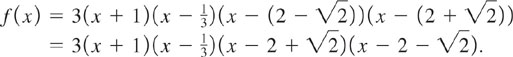
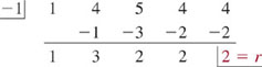
EXAMPLE 4 Example 1 Revisited
In Example 1 we demonstrated that ![]() is a zero of f(x) = 2x3 − 9x2 = 6x − 1.We now know that
is a zero of f(x) = 2x3 − 9x2 = 6x − 1.We now know that ![]() is a factor of f(x) and that f(x) has three zeros. The synthetic division
is a factor of f(x) and that f(x) has three zeros. The synthetic division
again demonstrates that ![]() is a zero of f(x) (the 0 remainder is the value of
is a zero of f(x) (the 0 remainder is the value of ![]() ) and, additionally, gives us the quotient q(x) obtained in the division of f(x) by
) and, additionally, gives us the quotient q(x) obtained in the division of f(x) by ![]() , that is,
, that is, ![]() . As shown in (8), we can now factor the quadratic quotient q(x) = 2x2 − 8x = 2 by finding the roots of 2x2 − 8x + 2 + 0 by the quadratic formula:
. As shown in (8), we can now factor the quadratic quotient q(x) = 2x2 − 8x = 2 by finding the roots of 2x2 − 8x + 2 + 0 by the quadratic formula:
Thus the remaining zeros of f(x) are the irrational numbers ![]() . With the identification of the leading coefficient as a3 = 2, it follows from (8) that the complete factorization of f(x) is then
. With the identification of the leading coefficient as a3 = 2, it follows from (8) that the complete factorization of f(x) is then
![]()
EXAMPLE 5 Using Synthetic Division
Find the complete factorization of
![]()
given that 1 is a zero of f of multiplicity two.
Solution We know that x − 1 is a factor of f(x), so by the division
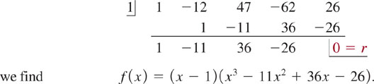
Since 1 is a zero of multiplicity 2, x − 1 must also be a factor of the quotient q(x) = x3 − 11x2 + 36x − 26. By the division,
we conclude that q(x) can be written q(x) = (x − 1)(x2 − 10x + 26). Therefore,
![]()
The remaining two zeros, found by solving x2 − 10x + 26 = 0 by the quadratic formula, are the complex numbers 5 + i and 5 − i. Since the leading coefficient is a4 = 1 the complete factorization of f(x) is
![]()
![]()
EXAMPLE 6 Complete Linear Factorization
Find a polynomial function f of degree three, with zeros 1, −4, and 5 such that its graph possesses the y-intercept (0, 5).
Solution Because we have three zeros 1, −4, and 5 we know x − 1, x + 4, and x − 5 are factors of f. However, the function we seek is not
![]()
The reason for this is that any nonzero constant multiple of f is a different polynomial with the same zeros. Notice, too, that the function in (9) gives f(0) = 20, but we want f(0) = 5. Hence we must assume that f has the form
![]()
where a is some real constant. Using (10), f(0) = 5 gives
![]()
and so ![]() . The desired function is then
. The desired function is then
![]()
![]()
We have seen in the introduction that the complex zeros of f(x) = x2 + 1 are i and −i. In Example 5 the complex zeros are 5 + i and 5 − i. In each case the complex zeros of the polynomial function are conjugate pairs. In other words, one complex zero is the conjugate of the other. This is no coincidence; complex zeros of polynomials with real coefficients always appear in conjugate pairs.
CONJUGATE ZEROS THEOREM
Let f(x) be a polynomial function of degree n > 1 with real coefficients. If z is a complex zero of f(x), then the conjugate ![]() is also a zero of f(x).
is also a zero of f(x).
EXAMPLE 7 Example 2 Revisited
In Example 2 we demonstrated that 1 + i is a complex zero of f(x) = x3 − 5x2 + 8x − 6. Since the coefficients of f are real numbers we conclude that another zero is the conjugate of 1 + i, namely, 1 − i. Thus we know two factors of f(x), x − (1 + i) and x − (1 + i). Carrying out the multiplication, we find
![]()
Thus we can write
![]()
We determine q(x) by performing the long division of f(x) by x2 − 2x + 2. (We can’t do synthetic division because we are not dividing by a linear factor.) From
we see that the complete factorization of f(x) is
![]()
The three zeros of f(x) are 1 + i, 1 − i, and 3.
![]()
3.3 Exercises
Answers to selected odd-numbered problems begin on page ANS–10.
In Problems 1–6, determine whether the indicated real number is a zero of the given polynomial function f. If yes, find all other zeros and then give the complete factorization of f(x).
1. 1; f(x) = 4x3 − 9x2 + 6x − 1
2. ![]()
3. 5; f(x) = x3 − 6x2 + 6x + 5
4. 3; f(x) = x3 − 3x2 + 4x − 12
5. ![]()
6.−2; f(x) = x3 − 4x2 − 2x + 20
In Problems 7–10, verify that each of the indicated numbers are zeros of the given polynomial function f. Find all other zeros and then give the complete factorization of f(x).
7. −3, 5; f(x) = 4x4 − 8x3 − 61x2 + 2x + 15
8. ![]()
9. ![]()
10. ![]()
In Problems 11–16, use synthetic division to determine whether the indicated linear polynomial is a factor of the given polynomial function f. If yes, find all other zeros and then give the complete factorization of f(x).
11. x − 5; f(x) = 2x2 + 6x − 25
12. ![]()
13. x − 1; f(x) = x3 + x − 2
14. ![]()
15. ![]()
16. x − 2; f(x) = x3 − 6x2 − 16x + 48
In Problems 17–20, use division to show that the indicated polynomial is a factor of the given polynomial function f. Find all other zeros and then give the complete factorization of f(x).
17. (x − 1)(x − 2); f(x) = x4 − 3x3 + 6x2 − 12x + 8
18. x(3x − 1); f(x) = 3x4 − 7x3 + 5x2 −x
19. (x − 1)2; f(x) = 2x4 + x3 − 5x2 −x + 3
20. (x + 3)2; f(x) = x4 − 4x3 − 22x2 + 84x + 261
In Problems 21–26, verify that the indicated complex number is a zero of the given polynomial function f. Proceed as in Example 7 to find all other zeros and then give the complete factorization of f(x).
21. 2i; f(x) = 3x3 − 5x2 + 12x − 20
22. ![]()
23. −1 + i; f(x) = 5x3 + 12x2 + 14x + 4
24. −i; f(x) = 4x4 − 8x3 + 9x2 − 8x + 5
25. 1 + 2i; f(x) = x4 − 2x3 − 4x2 + 18x − 45
26. 1 + i; f(x) = 6x4 − 11x3 + 9x2 + 4x − 2
In Problems 27–32, find a polynomial function f with real coefficients of the indicated degree that possesses the given zeros.
27. degree 4; 2, 1, −3 (multiplicity 2)
28. ![]()
29. degree 5; 3 + i, 0 (multiplicity 3)
30. degree 4; 5i, 2 − 3i
31. degree 2; 1 − 6i
32. degree 2; 4 + 3i
In Problems 33–36, find the zeros of the given polynomial function f. State the multiplicity of each zero.
33. f(x) = x(4x − 5)2(2x − 1)3
34. f(x) = x4 + 6x3 + 9x2
35. f(x) = (9x2 − 4)2
36. f(x) = (x2 + 25)(x2 − 5x + 4)2
In Problems 37 and 38, find the value(s) of k such that the indicated number is a zero of f(x). Then give the complete factorization of f(x).
37. 3; f(x) = 2x3 − 2x2 + k
38. 1; f(x) = x3 + 5x2 − k2x + k
In Problems 39 and 40, find a polynomial function f of the indicated degree whose graph is given in the figure.
39. degree 3
FIGURE 3.3.1 Graph for Problem 39
40. degree 5
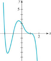
FIGURE 3.3.2 Graph for Problem 40
For Discussion
41. Discuss:
(a) For what positive-integer values of n is x − 1 a factor of f(x) = xn − 1?
(b) For what positive-integer values of n is x + 1 a factor of f(x) = xn + 1?
42. Suppose f(x) is a polynomial function of degree three with real coefficients. Why can’t f(x) have three complex zeros? Put another way, why must at least one zero of a cubic polynomial function be a real number? Can you generalize this result?
43. What is the smallest degree that a polynomial function f(x) with real coefficients can have such that 1 + i is a complex zero of multiplicity 2? Of multiplicity 3?
44. Let z = a + bi. Show that ![]() are real numbers.
are real numbers.
45. Let z = a + bi. Use the results of Problem 44 to show that
![]()
is a polynomial function with real coefficients.
3.4 Real Zeros of Polynomial Functions
![]() Introduction In the preceding section we saw that as a consequence of the Fundamental Theorem of Algebra, a polynomial function f of degree n has n zeros when the multiplicities of the zeros are counted. We also saw that a zero of a polynomial function could be either a real or a complex number. In this section we confine our attention to real zeros of polynomial functions with real coefficients.
Introduction In the preceding section we saw that as a consequence of the Fundamental Theorem of Algebra, a polynomial function f of degree n has n zeros when the multiplicities of the zeros are counted. We also saw that a zero of a polynomial function could be either a real or a complex number. In this section we confine our attention to real zeros of polynomial functions with real coefficients.
![]() Real Zeros If a polynomial function f of degree n > 0 has m (not necessarily distinct) real zeros c1, c2,…, cm, then by the Factor Theorem each of the linear polynomials x − c1, x − c2,…, x − cm are factors of f(x). That is,
Real Zeros If a polynomial function f of degree n > 0 has m (not necessarily distinct) real zeros c1, c2,…, cm, then by the Factor Theorem each of the linear polynomials x − c1, x − c2,…, x − cm are factors of f(x). That is,
![]()
where q(x) is a polynomial. Thus n, the degree of f, must be greater than or possibly equal to m, the number of real zeros when each is counted according to its multiplicity. Using slightly different words, we restate the last sentence.
NUMBERS OF REAL ZEROS
A polynomial function f of degree n > 0 has at most n real zeros (not necessarily distinct).
Let’s summarize some facts about real zeros of a polynomial function f of degree n:
•f may not have any real zeros.
For example, the fourth degree polynomial function f(x) = x4 + 9 has no real zeros, since there exists no real number x satisfying x4 + 9 + 0 or x4 = −9.
•f may have m real zeros where m < n.
For example, the third degree polynomial function f(x) = (x − 1)(x2 + 1) has one real zero.
•f may have n real zeros.
For example, by factoring the third degree polynomial function f(x) = x3 −x as f(x) = x(x2 − 1) + x(x + 1)(x − 1), we see that it has three real zeros.
•f has at least one real zero when n is odd.
This is a consequence of the fact that complex zeros of a polynomial functionf with real coefficients must appear in conjugate pairs. Thus if we write down an arbitrary cubic polynomial function such as f(x) = x3 + x + 1, we know thatf cannot have just one complex zero, nor can it have three complex zeros. Put another way, f(x) = x3 + x + 1 either has exactly one real zero or it has exactly three real zeros.
•If the coefficients of f(x) are positive and the constant term a0 ≠ 0, then any real zeros of f must be negative.
![]() Finding Real Zeros It is one thing to talk about the existence of real and complex zeros of a polynomial function; it is an entirely different problem to actually find these zeros. The problem of finding a formula that expresses the zeros of a general nth degree polynomial functionf in terms of its coefficients perplexed mathematicians for centuries. We have seen in Sections 2.4 and 3.3 that in the case of a second-degree, or quadratic, polynomial function f(x) = ax2 + bx + c, where the coefficients a, b, and c are real numbers, the zeros c1 and c2 of f can be found using the quadratic formula.
Finding Real Zeros It is one thing to talk about the existence of real and complex zeros of a polynomial function; it is an entirely different problem to actually find these zeros. The problem of finding a formula that expresses the zeros of a general nth degree polynomial functionf in terms of its coefficients perplexed mathematicians for centuries. We have seen in Sections 2.4 and 3.3 that in the case of a second-degree, or quadratic, polynomial function f(x) = ax2 + bx + c, where the coefficients a, b, and c are real numbers, the zeros c1 and c2 of f can be found using the quadratic formula.
The problem of finding zeros of third-degree, or cubic, polynomial functions was solved in the sixteenth century through the pioneering work of the Italian mathematician Niccolo Fontana (1499–1557), also known as Tartaglia—“the stammerer.” Around 1540 another Italian mathematician, Lodovico Ferrari (1522–1565) discovered an algebraic formula for determining the zeros for fourth degree, or quartic, polynomial functions. Since these formulas are complicated and difficult to use, they are seldom discussed in elementary courses.
For the next 284 years no one discovered any formulas for zeros for general polynomial functions of degrees five, six, …. For good reason! In 1824, at age 22, the Norwegian mathematician Niels Henrik Abel (1802–1829) proved it was impossible to find such formulas for the zeros of all general polynomials of degrees n ≥ 5 in terms of their coefficients.

Niels Henrik Abel
![]() Rational Zeros Real zeros of a polynomial function are either rational or irrational numbers. A rational number is a number of the form p/s, where p and s are integers and s ≠ 0. An irrational number is one that is not rational. For example,
Rational Zeros Real zeros of a polynomial function are either rational or irrational numbers. A rational number is a number of the form p/s, where p and s are integers and s ≠ 0. An irrational number is one that is not rational. For example, ![]() and −9 are rational numbers, but
and −9 are rational numbers, but ![]() and π are irrational, that is, neither
and π are irrational, that is, neither ![]() nor π can be written as a fraction p/s where p and s are integers. So how do we find real zeros for polynomial functions of degree n > 2? The bad news: For irrational real zeros, we may have to be content to use an accurate graph to “eyeball” their location on the x-axis and then use one of the many sophisticated methods for approximating the zero that have been developed over the years. The good news: We can always find the rational real zeros of any polynomial function with rational coefficients. We have already seen that synthetic division is a useful method for determining whether a given number c is a zero of a polynomial function f(x). When the remainder in the division of f(x) by x − c is r = 0, we have found a zero of the polynomial function f, since r = f(c) = 0. For example,
nor π can be written as a fraction p/s where p and s are integers. So how do we find real zeros for polynomial functions of degree n > 2? The bad news: For irrational real zeros, we may have to be content to use an accurate graph to “eyeball” their location on the x-axis and then use one of the many sophisticated methods for approximating the zero that have been developed over the years. The good news: We can always find the rational real zeros of any polynomial function with rational coefficients. We have already seen that synthetic division is a useful method for determining whether a given number c is a zero of a polynomial function f(x). When the remainder in the division of f(x) by x − c is r = 0, we have found a zero of the polynomial function f, since r = f(c) = 0. For example, ![]() is a zero of f(x) = 18x3 − 15x2 + 14x −8, since
is a zero of f(x) = 18x3 − 15x2 + 14x −8, since
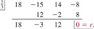
Hence by the Factor Theorem, both ![]() and the quotient 18x2 − 3x + 12 are factors off and so we can write the polynomial function as the product
and the quotient 18x2 − 3x + 12 are factors off and so we can write the polynomial function as the product
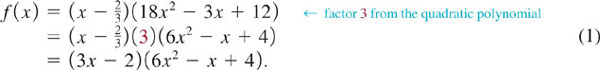
As discussed in the preceding section, if we can factor the polynomial to the point where the remaining factor is a quadratic polynomial, we can then find the remaining two zeros by the quadratic formula. For this example, the factorization in (1) is as far as we can go using real numbers since the zeros of the quadratic factor 6x2 −x + 4 are complex (verify). But the indicated multiplication in (1) illustrates something important about rational zeros. The leading coefficient 18 and the constant term −8 of f(x) are obtained from the products
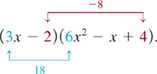
Thus we see that the denominator 3 of the rational zero ![]() is a factor of the leading coefficient 18 of f(x) = 18x3 − 15x2 + 14x − 8, and the numerator 2 of the rational zero is a factor of the constant term −8.
is a factor of the leading coefficient 18 of f(x) = 18x3 − 15x2 + 14x − 8, and the numerator 2 of the rational zero is a factor of the constant term −8.
This example illustrates the following general principle for determining the rational zeros of a polynomial function. Read the following theorem carefully; the coefficients of f are not only real numbers—they must be integers.
RATIONAL ZEROS THEOREM
Let p/s be a rational number in lowest terms and a zero of the polynomial function
![]()
where the coefficients an, an−1,…, a2, a1, a0 are integers with an ≠ 0. Then p is an integer factor of the constant term a0 and s is an integer factor of the leading coefficient an.
The Rational Zeros Theorem deserves to be read several times. Note that the theorem does not assert that a polynomial function f with integer coefficients must have a rational zero; rather, it states that if a polynomial function f with integer coefficients has a rational zero p/s, then necessarily:
![]()
By forming all possible quotients of each integer factor of a0 to each integer factor of an, we can construct a list of potential rational zeros of f.
EXAMPLE 1 Rational Zeros
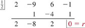
Find all rational zeros of f(x) = 3x4 − 10x3 − 3x2 + 8x − 2.
Solution We identify the constant term a0 = −2 and leading coefficient a4 = 3, and then list all the integer factors of a0 and a4, respectively:
![]()
Now we form a list of all possible rational zeros p/s by dividing all the factors of p by ±1 and then by ±3:
![]()
We know that the given fourth-degree polynomial functionf has four zeros; if any of these zeros is a real number and is rational, then it must appear in the list (2).
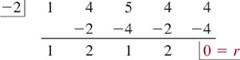
To determine which, if any, of the numbers in (2) are zeros, we could use direct substitution into f(x). Synthetic division, however, is usually a more efficient means of evaluating f(x). We begin by testing −1:
The zero remainder shows r = f(−1) = 0, and so −1 is a zero of f. Hence x − (−1) = x + 1 is a factor of f. Using the quotient found in (3) we can write
![]()
From (4) we see that any other rational zero off must be a zero of the quotient 3x3 − 13x2 + 10x − 2. Since the latter polynomial is of lower degree, it will be easier to use synthetic division on it rather than on f(x) to check the next rational zero. At this point in the process you should check to see whether the zero just found is a repeated zero. This is done by determining whether the found zero is also a zero of the quotient. A quick check, using synthetic division, shows that −1 is not a repeated zero of f since it is not a zero of 3x3 − 13x2 + 10x − 2. So we move on and determine whether the number 1 is a rational zero of f. Indeed, it is not because the division
shows that the remainder is r = −2 ≠ 0. Checking ![]() , we have
, we have
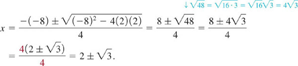
Thus ![]() is a zero. At this point we can stop using synthetic division since (6) indicates that the remaining factor of f is the quadratic polynomial 3x2 − 12x = 6. From the quadratic formula we find that the remaining real zeros are
is a zero. At this point we can stop using synthetic division since (6) indicates that the remaining factor of f is the quadratic polynomial 3x2 − 12x = 6. From the quadratic formula we find that the remaining real zeros are ![]() . Therefore the given polynomial function f has two rational zeros, −1 and
. Therefore the given polynomial function f has two rational zeros, −1 and ![]() , and two irrational zeros,
, and two irrational zeros, ![]() .
.
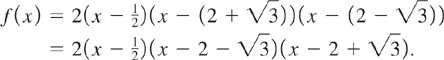
![]()
If you have access to technology, your selection of rational numbers to test in Example 1 can be motivated by a graph of the function f(x) = 3x4 − 10x3 − 3x2 + 8x − 2. With the aid of a graphing utility we obtain the graphs in FIGURE 3.4.1. In Figure 3.4.1(a) it would appear that f has at least three real zeros. But by “zooming-in” on the graph on the interval [0, 1], Figure 3.4.1(b) reveals that f actually has four real zeros: one negative and three positive. Thus, once you have determined one negative rational zero of f you may disregard all other negative numbers as potential zeros.
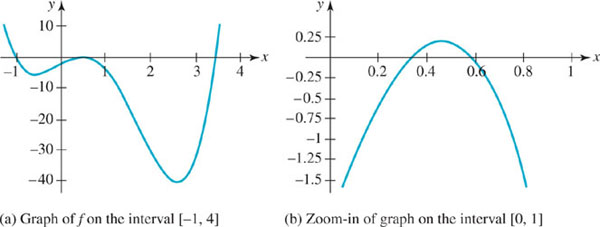
FIGURE 3.4.1 Graph of function f in Example 1
EXAMPLE 2 Complete Factorization
Since the function f in Example 1 is of degree 4 and we have found four real zeros, we can give its complete factorization. Using the leading coefficient a4 = 3, it follows from (6) of Section 3.3 that
![]()
EXAMPLE 3 Rational Zeros
Find all rational zeros of f(x) = x4 + 4x3 + 5x2 + 4x + 4.
Solution In this case the constant term is a0 = 4 and the leading coefficient is a4 = 1. The integer factors of a0 and a4 are, respectively:
![]()
The list of all possible rational zeros p/s is:
![]()
Since all the coefficients of f are positive, substituting a positive number from the foregoing list into f(x) can never result in f(x) = 0. Thus the only numbers that are potential rational zeros are −1, −2, and −4. From the synthetic division
we see that −1 is not a zero. However, from
we see −2 is a zero. We now test to see whether −2 is a repeated zero. Using the coefficients in the quotient,
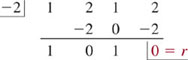
it follows that − 2 is a zero of multiplicity 2. So far we have shown that
![]()
Since the zeros of x2 + 1 are the complex conjugates i and −i, we can conclude that −2 is the only rational real zero of f(x).
![]()
EXAMPLE 4 No Rational Zeros
Consider the polynomial function f(x) = x5 − 4x − 1. The only possible rational zeros are −1 and 1, and it is easy to see that neither f(−1) nor f(1) are 0. Thus f has no rational zeros. Since f is of odd degree we know that it has at least one real zero, and so that zero must be an irrational number. With the aid of a graphing utility we obtain the graph in FIGURE 3.4.2. Note in the figure that the graph to the right of x = 2 cannot turnback down and the graph to the left of x = −2 cannot turn back up, so that the graph crosses the x-axis five times because that shape of the graph would be inconsistent with the end behavior of f. Thus we can conclude that the function f possesses three irrational real zeros and two complex conjugate zeros. The best we can do here is to approximate these zeros. Using a computer algebra system such as Mathematica we can approximate both the real and the complex zeros. We find these approximations to be −1.34, −0.25, 1.47, 0.061 = 1.42i, and 0.061 − 1.42i.
![]()
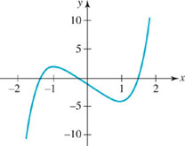
FIGURE 3.4.2 Graph off in Example 4
Although the Rational Zeros Theorem requires that the coefficients of a polynomial function f be integers, in some circumstances we can apply the theorem to a polynomial function with some real noninteger coefficients. The next example illustrates the concept.
EXAMPLE 5 Noninteger Coefficients
Find the rational zeros of ![]() .
.
Solution By multiplying f by the least common denominator 12 of all the rational coefficients, we obtain a new function g with integer coefficients:
![]()
In other words, g(x) = 12 f(x). If c is a zero of the function g, then c is also zero f because g(c) = 0 + 12 f(c) implies f(c) = 0. After working through the numbers in the list of potential rational zeros
![]()
we find that ![]() are zeros of g, and hence are rational zeros of f.
are zeros of g, and hence are rational zeros of f.
![]()
3.4 Exercises
Answers to selected odd-numbered problems begin on page ANS–10.
In Problems 1–20, find all rational zeros of the given polynomial function f.
1. f(x) = 5x3 − 3x2 + 8x + 4
2. f(x) = 2x3 + 3x2 −x + 2
3. f(x) = x3 − 8x − 3
4. f(x) = 2x3 − 7x2 − 17x + 10
5. f(x) = 4x4 − 7x2 + 5x − 1
6. f(x) = 8x4 − 2x3 + 15x2 − 4x − 2
7. f(x) = x4 + 2x3 + 10x2 + 14x + 21
8. f(x) = 3x4 + 5x2 + 1
9. f(x) = 6x4 − 5x3 − 2x2 − 8x + 3
10. f(x) = x4 + 2x3 − 2x2 − 6x − 3
11. f(x) = x4 + 6x3 − 7x
12. f(x) = x5 − 2x2 − 12x
13. f(x) = x5 + x4 − 5x3 + x2 − 6x
14. f(x) = 128x6 − 2
15. ![]()
16. f(x) = 0.2x3 −x + 0.8
17. f(x) = 2.5x3 + x2 + 0.6x + 0.1
18. ![]()
19. ![]()
20. ![]()
In Problems 21–30, find all real zeros of the given polynomial function f. Then factor f(x) using only real numbers.
21. f(x) = 8x3 +5x2 − 11x + 3
22. f(x) = 6x3 + 23x2 + 3x − 14
23. f(x) = 10x4 − 33x3 + 66x − 40
24. f(x) = x4 − 2x3 − 23x2 + 24x + 144
25.f(x) = x5 + 4x4 − 6x3 − 24x2 + 5x + 20
26. f(x) = 18x5 + 75x4 + 47x3 − 52x2 − 11x + 3
27. f(x) = 4x5 − 8x4 − 24x3 + 40x2 − 12x
28. f(x) = 6x5 + 11x4 − 3x3 − 2x2
29. f(x) = 16x5 − 24x4 + 25x3 + 39x2 − 23x + 3
30. f(x) = x6 − 12x4 + 48x2 − 64
In Problems 31–36, find all real solutions of the given equation.
31. 2x3 + 3x2 + 5x + 2 = 0
32. x3 − 3x2 = 24
33. 2x4 + 7x3 − 8x2 − 25x − 6 = 0
34. 9x4 + 21x3 + 22x2 + 2x − 4 = 0
35. x5 − 2x4 + 2x3 − 4x2 + 5x − 2 = 0
36. 8x4 − 6x3 − 7x2 + 6x − 1 = 0
In Problems 37 and 38, find a polynomial function f of the indicated degree with integer coefficients that possesses the given rational zeros.
37. degree 4; 24, ![]()
38. degree 5; 22, ![]() ,
,
39. Use the Intermediate Value Theorem (see Section 3.1) to show that the polynomial function f(x) = 4x3 − 11x2 + 14x − 6 has a zero in the interval [0, 1]. Find the zero.
40. List, but do not test, all possible rational zeros of
![]()
In Problems 41 and 42, find a cubic polynomial function f that satisfies the given conditions.
41. rational zeros 1 and 2, f(0) = 1 and f(−1) = 4
42. rational zero ![]() , irrational zeros
, irrational zeros ![]() , coefficient of x is 2
, coefficient of x is 2
Miscellaneous Calculus-Related Problems
43. Construction of a Box A box with no top is made from a square piece of cardboard by cutting square pieces from each corner and then folding up the sides. See FIGURE 3.4.3. The length of one side of the cardboard is 10 inches. Find the length of one side of the squares that were cut from the corners if the volume of the box is 48 in3.
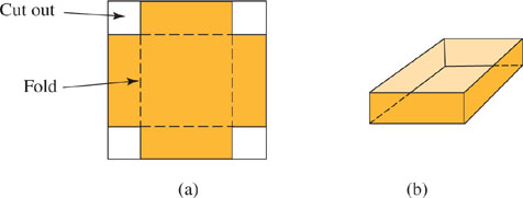
FIGURE 3.4.3 Box in Problem 43
44. Deflection of a Beam A cantilever beam 20 ft long with a load of 600 lb at its right end is deflected by an amount ![]() , where d is measured in inches and x in feet. See FIGURE 3.4.4. Find x when the deflection is 0.1215 in. When the deflection is 1 in.
, where d is measured in inches and x in feet. See FIGURE 3.4.4. Find x when the deflection is 0.1215 in. When the deflection is 1 in.
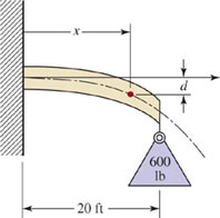
FIGURE 3.4.4 Cantilever beam in Problem 44
For Discussion
45. Discuss: What is the maximum number of times the graphs of the given polynomial functions can intersect?
(a) f(x) = a3x3 + a2x2 + a1x + a0, g(x) + b2x2 + b1x + b0
(b) f(x) = x3 + a2x2 + a1x + a0, g(x) + x3 + b2x2 + b1x + b0
46. Consider the polynomial function f(x) = xn + an−1xn−1 + … + a1x + a0, where the coefficients an−1, …, a1, a0 are nonzero even integers. Discuss why −1 and 1 cannot be zeros of f.
47. If the leading coefficient of a polynomial function f with integer coefficients is 1, then what can be said about the possible real zeros of f?
48. If k is a prime number (a positive integer greater than 1 whose only positive integer factors are itself and 1) such that k > 2, then what are the possible rational zeros of f(x) = 6x4 − 9x2 + k?
49. (a) The real number ![]() is a zero of the polynomial function f(x) = x2 − 2. How does the discussion in this section prove that
is a zero of the polynomial function f(x) = x2 − 2. How does the discussion in this section prove that ![]() is irrational?
is irrational?
(b) Use the idea implied in part (a) to prove that the real number ![]() is irrational.
is irrational.
50. Without doing any work, explain why the polynomial function
![]()
has no real zeros.
3.5 Rational Functions
![]() Introduction Many functions are built up out of polynomial functions by means of arithmetic operations and function composition (see Section 2.6). In this section we construct a class of functions by forming the quotient of two polynomial functions.
Introduction Many functions are built up out of polynomial functions by means of arithmetic operations and function composition (see Section 2.6). In this section we construct a class of functions by forming the quotient of two polynomial functions.
RATIONAL FUNCTION
A rational function y = f(x) is a function of the form
![]()
where P and Q are polynomial functions.
For example, the following functions are rational functions:
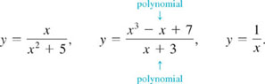
The function
![]()
is not a rational function. In (1) we cannot allow the denominator to be zero. So the domain of a rational function f(x) = P(x)/Q(x) is the set of all real numbers except those numbers for which the denominator Q(x) is zero. For example, the domain of the rational function f(x) = (2x3 − 1)/(x2 − 9) is {x|x ≠ − 3, x + 3} or (−∞, −3) ∪ (−3, 3) ∪ (3, ∞). It goes without saying that we also disallow the zero polynomial Q(x) = 0 as a denominator.
![]() Graphs Graphing a rational function f is a little more complicated than graphing a polynomial function because in addition to paying attention to
Graphs Graphing a rational function f is a little more complicated than graphing a polynomial function because in addition to paying attention to
- intercepts,
- symmetry, and
- shifting/reflecting/stretching of known graphs,
you should also keep an eye on
- the domain of f, and
- the degrees of P(x) and Q(x).
The latter two topics are important in determining whether a graph of a rational function possesses asymptotes.
The y-intercept is the point (0, f(0)), provided the number 0 is in the domain of f. For example, the graph of the rational function f(x) = (1 −x)/x does not cross the y-axis since f(0) is not defined. If the polynomials P(x) and Q(x) have no common factors, then the x-intercepts of the graph of the rational function f(x) = P(x)/Q(x) are the points whose x-coordinates are the real zeros of the numerator P(x). In other words, the only way we can have f(x) = P(x)/Q(x) + 0 is to have P(x) = 0. The graph of a rational function f is symmetric with respect to the y-axis if f (−x) = f(x), and symmetric with respect to the origin if f (−x) = − f(x)Since it is easy to spot an even or an odd polynomial function (see page 131), here is an easy way to determine symmetry of the graph of a rational function. We again assume P(x) and Q(x) have no common factors.
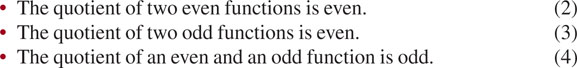
See Problem 48 in Exercises 3.5.
We have already seen the graphs of two simple rational functions, y = 1/x and y = 1/x2, in Figures 2.2.1(e) and 2.2.1(f). You are encouraged to review those graphs at this time. Note that P(x) = 1 is an even function and Q(x) = x is an odd function, so y = 1/x is an odd function by (4). On the other hand, P(x) = 1 is an even function and Q(x) = x2 is an even function, so y = 1/x2 is an even function by (2).
EXAMPLE 1 Shifted Reciprocal Function
Graph the function ![]() .
.
Solution The graph possesses no symmetry since Q(x) = x − 1 is neither even nor odd. Since f(0) = −2, the y-intercept is (0, −2). Because P(x) = 2 is never 0, there are no x-intercepts. You might also recognize that the graph of this rational function is the graph of the reciprocal function y = 1/x stretched vertically by a factor of 2 and shifted 1 unit to the right. The point (1, 1) is on the graph of y = 1/x; in FIGURE 3.5.1, after the vertical stretch and horizontal shift, the corresponding point on the graph of y = 2/(x − 1) is (2, 2).
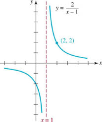
FIGURE 3.5.1 Graph of function in Example 1
The vertical line x = 1 and the horizontal line y = 0 (the equation of the x-axis) are of special importance for this graph.
The vertical dashed line x = 1 in Figure 3.5.1 is the y-axis in Figure 2.2.1(e) shifted 1 unit to the right. Although the number 1 is not in the domain of the given function, we can evaluate f at values of x that are near 1. For example, you should verify that
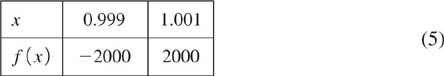
The table in (5) shows that for values of x close to 1, the corresponding function values f(x) are large in absolute value. On the other hand, for values of x for which | x | is large, the corresponding function values f(x) are near 0. For example, you should verify that
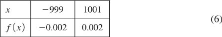
Geometrically, as x approaches 1, the graph of the function approaches the vertical line x = 1, and as |x| increases without bound the graph of the function approaches the horizontal line y = 0.
![]()
![]() Asymptotes Recall from Section 1.5 that to indicate that x is approaching a number a, we use the notation
Asymptotes Recall from Section 1.5 that to indicate that x is approaching a number a, we use the notation
•x → a− to mean that x is approaching a from the left, that is, through numbers that are less than a;
•x → a+ to mean that x is approaching a from the right, that is, through numbers that are greater than a; and
•x → a to mean that x is approaching a from both the left and the right.
We also use the infinity symbols and the notation
•x → − ∞ to mean that x becomes unbounded in the negative direction, and
•x →∞ to mean that x becomes unbounded in the positive direction.
Similar interpretations are given to the symbols f(x)→ −∞ and f(x) → ∞. These notational devices are a convenient way of describing the behavior of a function either near a number x = a or as x increases to the right or decreases to the left. Thus, in Example 1 it is apparent from (5) and Figure 3.5.1 that
![]()
In words, the notation in the preceding line signifies that the function values are decreasing without bound as x approaches 1 from the left, and the function values are increasing without bound as x approaches 1 from the right. From (6) and Figure 3.5.1 it should also be apparent that
![]()
In Figure 3.5.1, the vertical line whose equation is x = 1 is a called a vertical asymptote for the graph of f, and the horizontal line whose equation is y = 0 is called a horizontal asymptote for the graph of f.
In this section we will examine three types of asymptotes, which correspond to the three types of lines studied in Section 2.3: vertical lines, horizontal lines, and slant (or oblique) lines. The characteristic of any asymptote is that the graph of a function f must get close to, or approach, the line.
VERTICAL ASYMPTOTE
A line x = a is said to be a vertical asymptote for the graph of a function f if at least one of the following six statements is true:
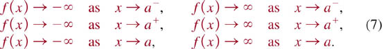
FIGURE 3.5.2 illustrates four of the possibilities listed in (7) for the unbounded behavior of a function f near a vertical asymptote x = a. If the function exhibits the same kind of unbounded behavior from both sides of x = a, then we write either
![]()
In Figure 3.5.2(d) we see that f(x) → ∞ as x → a− and f(x) → ∞ as x → a+, and so we write f(x) → ∞ as x → a.
FIGURE 3.5.2 The line x = a is a vertical asymptote
If x = a is a vertical asymptote for the graph of a rational function f(x) = P(x)/Q(x), then the function values f(x) become unbounded as x approaches a from both sides, that is, from the right (x → a+) and from the left (x → a−). The graphs in Figures 3.5.2(c) and 3.5.2(d) (or the reflection of these graphs in the x-axis) are typical graphs of a rational function with a single vertical asymptote. As can be seen from these figures, a rational function with a vertical asymptote is a discontinuous function. There is an infinite break in each graph at x = a. As seen in Figures 3.5.2(c) and 3.5.2(d), a single vertical asymptote divides the xy-plane into two regions, and within each region there is a single piece or branch of the graph of the rational function f.
HORIZONTAL ASYMPTOTE
A line y = c is said to be a horizontal asymptote for the graph of a function f if
![]()
In FIGURE 3.5.3 we have illustrated some typical horizontal asymptotes. We note, in conjunction with Figure 3.5.3(d) that, in general, the graph of a function can have at most two horizontal asymptotes, but the graph of a rational function f(x) = P(x)/Q(x) can have at most one. If the graph of a rational function f possesses a horizontal asymptote y = c, then as shown in Figure 3.5.3(c),
![]()
![]() Remember this.
Remember this.
FIGURE 3.5.3 The line y = c is a horizontal asymptote in (a), (b), and (c)
The last line is a mathematical description of the end behavior of the graph of a rational function with a horizontal asymptote. Also, the graph of a function can never cross a vertical asymptote but, as suggested in Figure 3.5.3(a), a graph can cross a horizontal asymptote.
SLANT ASYMPTOTE
A line y = mx + b, m ≠ 0, is said to be a slant asymptote for the graph of a function f if

![]() A slant asymptote is also called an oblique asymptote.
A slant asymptote is also called an oblique asymptote.
The notation in (11) means that the graph of f possesses a slant asymptote whenever the function values f(x) become closer and closer to the values of y on the line y = mx + b as x becomes large in absolute value. Another way of stating (11) is: A line y = mx + b is a slant asymptote for the graph of f if the vertical distance d(x) between points with the same x-coordinate on the two graphs satisfies
![]()
See FIGURE 3.5.4. We note that if a graph of a rational function f(x) = P(x)/Q(x) possesses a slant asymptote it can have vertical asymptotes, but the graph cannot have a horizontal asymptote.
FIGURE 3.5.4 Slant asymptote is y = mx + b
On a practical level, vertical and horizontal asymptotes of the graph of a rational function f can be determined by inspection. So for the sake of discussion let us suppose that
![]()
represents a general rational function.
![]() Finding Vertical Asymptotes Let us assume that the polynomial functions P(x) and Q(x) in (12) have no common factors. In that case:
Finding Vertical Asymptotes Let us assume that the polynomial functions P(x) and Q(x) in (12) have no common factors. In that case:
• If a is a real number such that Q(a) = 0, then the line x = a is a vertical asymptote for the graph of f.
Since Q(x) is a polynomial function of degree m, it can have up to m real zeros, and so the graph of a rational function f can have up to m vertical asymptotes. If the graph of a rational function f has, say, k(k ≤ m) vertical asymptotes, then the k vertical lines divide the xy-plane into k = 1 regions. Thus the graph of this rational function would have k = 1 branches.
EXAMPLE 2 Vertical Asymptotes
(a) Inspection of the rational function , ![]() shows that the denominator Q(x) = x2 − 4 + (x + 2)(x − 2) + 0 at x = −2 and x = 2. These are equations of vertical asymptotes for the graph of f. The graph of f has three branches: one to the left of the line x = −2, one between the lines x = −2 and x = 2, and one to the right of the line x = 2.
shows that the denominator Q(x) = x2 − 4 + (x + 2)(x − 2) + 0 at x = −2 and x = 2. These are equations of vertical asymptotes for the graph of f. The graph of f has three branches: one to the left of the line x = −2, one between the lines x = −2 and x = 2, and one to the right of the line x = 2.
(b) The graph of the rational function ![]() has no vertical asymptotes, since Q(x) = x2 + x + 4 ≠ 0 for all real numbers.
has no vertical asymptotes, since Q(x) = x2 + x + 4 ≠ 0 for all real numbers.
![]()
![]() Finding Horizontal Asymptotes When we discussed end behavior of a polynomial function P(x) of degree n, we pointed out that P(x) behaves like y = anxn, that is, P(x) = anxn, for values of x large in absolute value. As a consequence, we see from
Finding Horizontal Asymptotes When we discussed end behavior of a polynomial function P(x) of degree n, we pointed out that P(x) behaves like y = anxn, that is, P(x) = anxn, for values of x large in absolute value. As a consequence, we see from
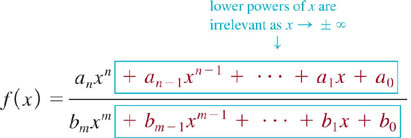
that f(x) behaves like ![]() for x → ± ∞.
for x → ± ∞.
Therefore:
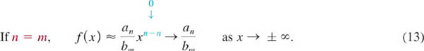
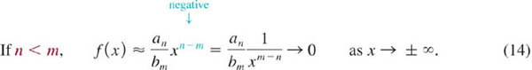
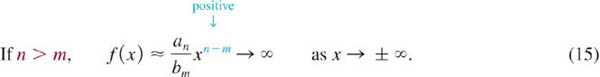
From (13), (14), and (15) we glean the following three facts about horizontal asymptotes for the graph of f(x) = P(x)/Q(x):
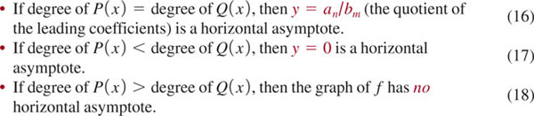
EXAMPLE 3 Horizontal Asymptotes
Determine whether the graph of each of the following rational functions possesses a horizontal asymptote.
(a) ![]()
(b) ![]()
(c) ![]()
Solution
(a) Since the degree of the numerator 3x2 + 4x − 1 is the same as the degree of the denominator 8x2 + x (both degrees are 2), we see from (13) that
![]()
As summarized in (16), ![]() is a horizontal asymptote for the graph of f.
is a horizontal asymptote for the graph of f.
(b) Since the degree of the numerator 4x3 + 7x + 8 is 3 and the degree of the denominator 2x4 + 3x2 −x + 6 is 4 (and 3 < 4), we see from (14) that
![]()
As summarized in (17), y = 0 (the x-axis) is a horizontal asymptote for the graph of f.
(c) Since the degree of the numerator 5x3 + x2 − 1 is 3 and the degree of the denominator 2x + 3 is 1 (and 3 > 1), we see from (15) that
![]()
As summarized in (18), the graph of f has no horizontal asymptote.
![]()
In the graphing examples that follow we will assume that P(x) and Q(x) in (12) have no common factors.
EXAMPLE 4 Graph of a Rational Function
Graph the function ![]() .
.
Solution Here are some things we look at to sketch the graph of f.
Symmetry: No symmetry. P(x) = 3 − x and Q(x) = x + 2 are neither even nor odd.
Intercepts: ![]() and so the y-intercept is
and so the y-intercept is ![]() . Setting P(x) = 0 or 3 − x = 0 implies 3 is a zero of P. The single x-intercept is (3, 0).
. Setting P(x) = 0 or 3 − x = 0 implies 3 is a zero of P. The single x-intercept is (3, 0).
Vertical Asymptotes: Setting Q(x) = 0 or x + 2 + 0 gives x = −2. The line x = −2 is a vertical asymptote.
Branches: Because there is only a single vertical asymptote, the graph of f consists of two distinct branches, one to the left of x = −2 and one to the right of x = −2.
Horizontal Asymptote: The degree of P and the degree of Q are the same (namely, 1), and so the graph of f has a horizontal asymptote. By rewriting f as ![]() we see that the ratio of leading coefficients is −1/1 = −1. From (16) we see that the line y = −1 is a horizontal asymptote.
we see that the ratio of leading coefficients is −1/1 = −1. From (16) we see that the line y = −1 is a horizontal asymptote.
The Graph: We draw the vertical and horizontal asymptotes using dashed lines. The right branch of the graph of f is drawn through the intercepts ![]() and (3, 0) in such a manner that it approaches both asymptotes. The left branch is drawn below the horizontal asymptote y = −1. Were we to draw this branch above the horizontal asymptote it would have to be near the horizontal asymptote from above and near the vertical asymptote from the left. In order to do this the branch of the graph would have to cross the x-axis, but since there are no more x-intercepts this is impossible. See FIGURE 3.5.5.
and (3, 0) in such a manner that it approaches both asymptotes. The left branch is drawn below the horizontal asymptote y = −1. Were we to draw this branch above the horizontal asymptote it would have to be near the horizontal asymptote from above and near the vertical asymptote from the left. In order to do this the branch of the graph would have to cross the x-axis, but since there are no more x-intercepts this is impossible. See FIGURE 3.5.5.
![]()
EXAMPLE 5 Example 4 Using Transformations
Long division and rigid transformations can sometimes be aids in graphing rational functions. Note that if we carry out the long division for the function f in Example 4, we see that
![]()
Thus, starting with the graph of y = 1/x, we stretch it vertically by a factor of 5. Next, shift the graph of y = 5/x two units to the left. Finally, shift y = 5/(x + 2) one unit vertically downward. You should verify that the net result is the graph in Figure 3.5.5.
![]()
EXAMPLE 6 Graph of a Rational Function
Graph the function ![]() .
.
Solution
Symmetry: Since P(x) = x is odd and Q(x) = 1 − x2 is even, the quotient P(x)/Q(x) is odd. The graph of f is symmetric with respect to the origin.
Intercepts: f(0) = 0, and so the y-intercept is (0, 0). Setting P(x) = x + 0 gives x = 0. Thus the only intercept is (0, 0).
Vertical Asymptotes: Setting Q(x) = 0 or 1 − x2 = 0 = 0 gives x = − 1 and x = 1. The lines x = −1 and x = 1 are vertical asymptotes.
Branches: Because there are two vertical asymptotes, the graph of f consists of three distinct branches, one to the left of the line x = −1, one between the lines x = −1 and x = 1, and one to the right of the line x = 1.
Horizontal Asymptote: Since the degree of the numerator x is 1 and the degree of the denominator 1 −x2 is 2 (and 1 < 2), it follows from (14) and (17) that y = 0 is a horizontal asymptote for the graph of f.
The Graph: We can plot the graph for x ≥ 0 and then use symmetry to obtain the remaining part of the graph of x = 0. We begin by drawing the vertical asymptotes using dashed lines. The half-branch of the graph of f on the interval [0, 1) is drawn starting at (0, 0). The function f must then increase because P(x) = x + 0, and Q(x) = 1 −x 2 + 0 indicates that f(x) > 0 for 0 < x < 1. This implies that near the vertical asymptote x = 1, f(x) → ∞ as x → 1−. The branch of the graph for x = 1 is drawn below the horizontal asymptote y = 0, since P(x) = x + 0 and Q(x) = 1 −x2 + 0 imply f(x) = 0. Thus f(x) → −∞ as x → 1 + and f(x) → 0 as x → ∞. The remainder of the graph for x = 0 is obtained by reflecting the graph for x = 0 through the origin. See FIGURE 3.5.6.
![]()
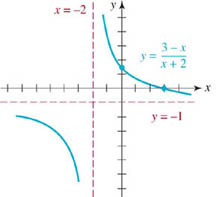
FIGURE 3.5.5 Graph of function in Example 4
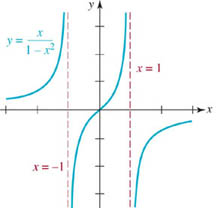
FIGURE 3.5.6 Graph of function in Example 6
EXAMPLE 7 Graph of a Rational Function
Graph the function ![]() .
.
Solution The given function f is similar to the function in Example 6 in that f is an odd function, (0, 0) is the only intercept of its graph, and its graph has the horizontal asymptote y = 0. However, note that since 1 + x2 > 0 for all real numbers, there are no vertical asymptotes. Thus there are no branches; the graph is one continuous curve. For x ≥ 0, the graph passes through (0, 0) and then must increase since f(x) > 0 for x > 0. Also, f must attain a relative maximum and then decrease in order to satisfy the condition f(x) → 0 as x → ∞. As mentioned in Section 3.1, the exact value of this relative maximum can be obtained through calculus techniques. Finally, we reflect the portion of the graph for x > 0 through the origin. The graph must look something like that shown in FIGURE 3.5.7.
![]()
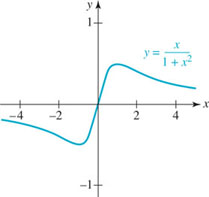
FIGURE 3.5.7 Graph of function in Example 7
![]() Finding Slant Asymptotes Let us again assume that the polynomials P(x) and Q(x) in (12) have no common factors. In that case we can recognize the existence of a slant asymptote in the following manner:
Finding Slant Asymptotes Let us again assume that the polynomials P(x) and Q(x) in (12) have no common factors. In that case we can recognize the existence of a slant asymptote in the following manner:
- If the degree of P (x) is precisely one greater than the degree of Q(x), that is, if the degree of Q(x) is m and the degree of P(x) is m + 1, then the graph of f possesses a slant asymptote.
We find the slant asymptote by division. Using long division to divide P(x) by Q(x) yields a quotient that is a linear polynomial mx + b and a polynomial remainder R(x):
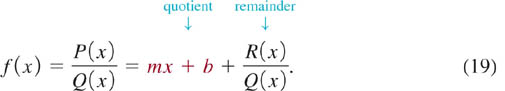
Because the degree of R(x) must be less than the degree of the divisor Q(x), we have R(x)/Q(x) → 0 as x → −∞ and as x → ∞, and consequently
![]()
In other words, an equation of the slant asymptote is y = mx + b, where mx + b is the quotient in (19).
If the denominator Q(x) is a linear polynomial, we can then use synthetic division to carry out the long division.
EXAMPLE 8 Graph with a Slant Asymptote
Graph the function ![]() .
.
Solution
Symmetry: No symmetry. P(x) = x2 −x − 6 and Q(x) = x − 5 are neither even nor odd.
Intercepts:![]() , and so the y-intercept is
, and so the y-intercept is ![]() . Setting P(x) = 0 or x2 −x − 6 + 0 or (x + 2)(x − 3) = 0 shows that −2 and 3 are zeros of P(x). The x-intercepts are (−2, 0) and (3, 0).
. Setting P(x) = 0 or x2 −x − 6 + 0 or (x + 2)(x − 3) = 0 shows that −2 and 3 are zeros of P(x). The x-intercepts are (−2, 0) and (3, 0).
Vertical Asymptotes: Setting Q(x) = 0 or x − 5 = 0 gives x = 5. The line x = 5 is a vertical asymptote.
Branches: The graph of f consists of two branches, one to the left of x = 5 and one to the right of x = 5.
Horizontal Asymptote: None.
Slant Asymptote: Since the degree of P(x) = x2 −x − 6 (which is 2) is exactly one greater than the degree of Q(x) = x − 5 (which is 1), the graph of f(x) has a slant asymptote. To find it, we divide P(x) by Q(x). Because Q(x) is a linear polynomial we can use synthetic division:
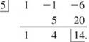
Recall that the latter notation means that
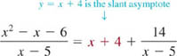
Note again that 14/(x − 5) → 0 as x → ± ∞. Hence the line y = x + 4 is a slant asymptote.
The Graph: Using the foregoing information we obtain the graph in FIGURE 3.5.8. The asymptotes are the dashed lines in the figure.
![]()
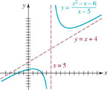
FIGURE 3.5.8 Graph of function in Example 8
EXAMPLE 9 Graph with a Slant Asymptote
By inspection it should be apparent that the graph of the rational function ![]() possesses a slant asymptote but no vertical asymptotes. Since the denominator is a quadratic polynomial we resort to long division to obtain
possesses a slant asymptote but no vertical asymptotes. Since the denominator is a quadratic polynomial we resort to long division to obtain
![]()
The slant asymptote is the line y = x. The graph has no symmetry. The y-intercept is 10, 122. The lack of vertical asymptotes indicates that the function f is continuous; its graph consists of an unbroken curve. Because the numerator is a polynomial of odd degree, we know that it has at least one real zero. Since x3 − 8x + 12 = 0 has no rational roots, we use approximation or graphical techniques to show that the equation possesses only one real irrational root. Thus the x-intercept is approximately (−3.4, 0). The graph of f is given in FIGURE 3.5.9. Notice in the figure that the graph of f crosses the slant asymptote.
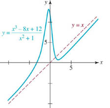
FIGURE 3.5.9 Graph of function in Example 9
![]()
![]() Graph with a Hole We assumed throughout the preceding discussion of asymptotes of rational functions that the polynomial functions P(x) and Q(x) in (1) have no common factors. We now know that if a is a real number such that Q(a) = 0, and P(x) and Q(x) have no common factors, then the line x = a is a vertical asymptote for the graph of f. Because Q is a polynomial function, it follows from the Factor Theorem that Q(x) = (x − a)q(x). The assumption that the numerator P and denominator Q have no common factors tells us that x − a is not a factor of P and so P(a) ≠ 0. When P(a) = 0and Q(a) = 0, then x + a may not be a vertical asymptote. For example, when a is a simple zero of both P and Q, then x = a is not a vertical asymptote for the graph of f(x) = P(x)/Q(x). To see this, we know from the Factor Theorem that if P(a) = 0 and Q(a) = 0, then x − a is a common factor of P and Q:
Graph with a Hole We assumed throughout the preceding discussion of asymptotes of rational functions that the polynomial functions P(x) and Q(x) in (1) have no common factors. We now know that if a is a real number such that Q(a) = 0, and P(x) and Q(x) have no common factors, then the line x = a is a vertical asymptote for the graph of f. Because Q is a polynomial function, it follows from the Factor Theorem that Q(x) = (x − a)q(x). The assumption that the numerator P and denominator Q have no common factors tells us that x − a is not a factor of P and so P(a) ≠ 0. When P(a) = 0and Q(a) = 0, then x + a may not be a vertical asymptote. For example, when a is a simple zero of both P and Q, then x = a is not a vertical asymptote for the graph of f(x) = P(x)/Q(x). To see this, we know from the Factor Theorem that if P(a) = 0 and Q(a) = 0, then x − a is a common factor of P and Q:
![]()
where p and q are polynomials such that p(a) ≠ 0and q(a) ≠ 0. After canceling
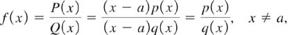
we see that f(x) is undefined at a, but the function values f(x) do not become unbounded as x → a− or as x → a+ because q(x) is not approaching 0. As an example, we saw in Section 2.5 that the graph of the rational function
![]()
is basically a straight line. But since f(2) is undefined there is no point (2, f(2)) on the line. Instead, there is a hole in the graph at the point (2, 4). See Figure 2.5.5(a).
EXAMPLE 10 Graph with a Hole
Graph the function ![]() .
.
Solution Although x2 −1 = 0 for x = −1 and x = 1, only x = 1 is a vertical asymptote. Note that the numerator P(x) and denominator Q(x) have the common factor x + 1, which we cancel provided x ≠ −1:
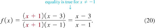
Thus we see from (20) that there is no infinite break in the graph at x = −1. We graph
![]() , by observing that the y-intercept is (0, 3), an x-intercept is (3, 0), a vertical asymptote is x = 1, and a horizontal asymptote is y = 1. The graph of this function has two branches, but the branch to the left of the vertical asymptote x = 1 has hole in it corresponding to the point (−1, 2). See FIGURE 3.5.10.
, by observing that the y-intercept is (0, 3), an x-intercept is (3, 0), a vertical asymptote is x = 1, and a horizontal asymptote is y = 1. The graph of this function has two branches, but the branch to the left of the vertical asymptote x = 1 has hole in it corresponding to the point (−1, 2). See FIGURE 3.5.10.
![]()
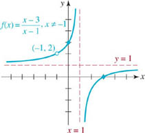
FIGURE 3.5.10 Graph of function in Example 10
NOTES FROM THE CLASSROOM
When asked whether they have ever heard the statement “An asymptote is a line that the graph approaches but does not cross,” a surprising number of students will raise their hands. First, let’s make it clear that the statement is false; a graph can cross a horizontal asymptote and can cross a slant asymptote. A graph can never cross a vertical asymptote x = a, since the function is inherently undefined at x = a. We can even find the points where a graph crosses a horizontal or slant asymptote. For example, the rational function ![]() as the horizontal asymptote y = 1. Determining whether the graph of f crosses the horizontal line y = 1 is equivalent to asking whether y = 1 is in the range of the function f. Setting f(x) equal to 1, that is,
as the horizontal asymptote y = 1. Determining whether the graph of f crosses the horizontal line y = 1 is equivalent to asking whether y = 1 is in the range of the function f. Setting f(x) equal to 1, that is,
Since ![]() is in the domain of f, the graph off crosses the horizontal asymptote at
is in the domain of f, the graph off crosses the horizontal asymptote at ![]() . Observe in Example 9 we can find the point where the slant asymptote crosses the graph of y = x by solving f(x) = x. You should verify that the point of intersection is
. Observe in Example 9 we can find the point where the slant asymptote crosses the graph of y = x by solving f(x) = x. You should verify that the point of intersection is ![]() . See Problems 31–36 in Exercises 3.5.
. See Problems 31–36 in Exercises 3.5.
3.5 Exercises
Answers to selected odd-numbered problems begin on page ANS–10.
In Problems 1 and 2, use a calculator to fill out the given table for the rational function ![]() .
.
1. x = 3 is a vertical asymptote for the graph of f
2. y = 2 is a horizontal asymptote for the graph of f
In Problems 3–22, find the vertical and horizontal asymptotes for the graph of the given rational function. Find x- and y-intercepts of the graph. Sketch the graph of f.
3. ![]()
4. ![]()
5. ![]()
6. ![]()
7. ![]()
8. ![]()
9. ![]()
10. ![]()
11. ![]()
12. ![]()
13. ![]()
14. ![]()
15. ![]()
16. ![]()
17. ![]()
18. ![]()
19. ![]()
20. ![]()
21. ![]()
22. ![]()
In Problems 23–30, find the vertical and slant asymptotes for the graph of the given rational function. Find x- and y-intercepts of the graph. Sketch the graph f.
23. ![]()
24. ![]()
25. ![]()
26. ![]()
27. ![]()
28. ![]()
29. ![]()
30. ![]()
In Problems 31–34, find the point where the graph of f crosses its horizontal asymptote. Sketch the graph of f.
31. ![]()
32. ![]()
33. ![]()
34. ![]()
In Problems 35 and 36, find the point where the graph of f crosses its slant asymptote. Use a graphing utility to obtain the graph of f and the slant asymptote in the same coordinate plane.
35. ![]()
36. ![]()
In Problems 37–40, find a rational function that satisfies the given conditions. There is no unique answer.
37. vertical asymptote: x = 2 horizontal asymptote: y = 1x-intercept: (5, 0)
38. vertical asymptote: x = 1 horizontal asymptote: y = −2 y-intercept: (0, −1)
39. vertical asymptotes: x = −1, x = 2 horizontal asymptote: y = 3 x-intercept: (3, 0)
40. vertical asymptote: x = 4 slant asymptote: y = x + 2
In Problems 41–44, find the asymptotes and any holes in the graph of the given rational function. Find x- and y-intercepts of the graph. Sketch the graph f.
41. ![]()
42. ![]()
43. ![]()
44. ![]()
Miscellaneous Applications
45. Parallel Resistors A 5-ohm resistor and a variable resistor are placed in parallel as shown in FIGURE 3.5.11. The resulting resistance R (in ohms) is related to the resistance r (in ohms) of the variable resistor by the equation
![]()
Sketch the graph of R as a function of r for r > 0. What is the resulting resistance R as r becomes very large?
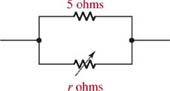
FIGURE 3.5.11 Parallel resistors in Problem 45
46. Power The electrical power P produced by a certain source is given by
![]()
where E is the voltage of the source, R is the resistance of the source, and r is the resistance in the circuit. Sketch the graph of P as a function of r using the values E = 5 volts and R = 1 ohm.
47. Illumination Intensity The intensity of illumination from a light source at any point is directly proportional to the strength of the source and inversely proportional to the square of the distance from the source. Given two sources of strengths 16 units and 2 units that are 100 cm apart, as shown in FIGURE 3.5.12, the intensity I at any point P between them is given by
![]()
where x is the distance from the 16-unit source. Sketch the graph of I(x) on the interval (0, 100). Describe the behavior of I(x) as x → 0+. As x → 100−.
FIGURE 3.5.12 Two light sources in Problem 47
For Discussion
48. Suppose f(x) = P(x)/Q(x). Prove the symmetry rules (2), (3), and (4) for rational functions.
49. Construct a rational function f(x) = P(x)/Q(x) whose graph crosses its slant asymptote twice.
50. If you have studied Section 1.5, then discuss how topics in this section and Section 3.2 can be used to help find the limit: ![]() .
.
3.6 Partial Fractions
![]() Introduction When two rational functions, say,
Introduction When two rational functions, say, ![]() , are added, the terms are combined by means of a common denominator:
, are added, the terms are combined by means of a common denominator:

Adding numerators on the right-hand side of (1) yields the single rational expression
![]()
An important procedure in the study of integral calculus requires that we be able to reverse the process. In other words, we would start with a rational expression such as (2) and then break it down, or decompose it, into simpler component fractions 2/(x + 5) and 1/(x + 1), called partial fractions.
![]() Partial Fractions The algebraic process for breaking down a rational expression such as (2) into partial fractions is known as partial fraction decomposition. For convenience we will assume that the rational function P(x)/Q(x), Q(x) ≠ 0, is a proper fraction or proper rational expression, that is, the degree of P(x) is less than the degree of Q(x). We will also assume once again that the polynomials P(x) and Q(x) have no common factors.
Partial Fractions The algebraic process for breaking down a rational expression such as (2) into partial fractions is known as partial fraction decomposition. For convenience we will assume that the rational function P(x)/Q(x), Q(x) ≠ 0, is a proper fraction or proper rational expression, that is, the degree of P(x) is less than the degree of Q(x). We will also assume once again that the polynomials P(x) and Q(x) have no common factors.
In the discussion that follows we consider four cases of partial fraction decomposition of P(x)/Q(x). The cases depend on the factors in the denominator Q(x). When the polynomial Q(x) is factored as a product of (ax + b)n and (ax2 + bx + c)m, n = 1, 2, …, m = 1, 2, …, where the coefficients a, b, and c are real numbers and the quadratic polynomial ax2 + bx + c is irreducible over the real numbers (that is, does not factor using real numbers), the rational expression P(x)/Q(x) can be decomposed into a sum of partial fractions of the form
![]()
CASE 1: Q(x) Contains Only Nonrepeated Linear Factors
We state the following fact from algebra without proof. If the denominator can be factored completely into linear factors,
![]()
where all the aix = bi, i = 1, 2,…, n are distinct (that is, no two factors are the same), then unique real constants C1, C2,…, Cn can be found such that

In practice we will use the letters A, B, C, …, in place of the subscripted coefficients C1, C2, C3,…. The next example illustrates this first case.
EXAMPLE 1 Distinct Linear Factors
To decompose ![]() into individual partial fractions we make the assumption, based on the form given in (3), that the rational function can be written as
into individual partial fractions we make the assumption, based on the form given in (3), that the rational function can be written as
![]()
We now clear (4) of fractions; this can be done by either combining the terms on the right-hand side of the equality over a least common denominator and equating numerators or by simply multiplying both sides of the equality by the denominator (x − 1)(x + 3) on the left-hand side. Either way, we arrive at
![]()
Multiplying out the right-hand side of (5) and grouping by powers of x gives
![]()
Each of the equations (5) and (6) is an identity, which means that the equality is true for all real values of x. As a consequence, the coefficients of x on the left-hand side of (6) must be the same as the coefficients of the corresponding powers of x on the right-hand side, that is,
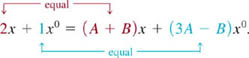
The result is a system of two equations in two unknowns A and B:
![]()
By adding the two equations we get 3 = 4A, and so we find that ![]() . Substituting this value into either equation in (7) then yields
. Substituting this value into either equation in (7) then yields ![]() . Hence the desired decomposition is
. Hence the desired decomposition is
![]()
You are encouraged to verify the foregoing result by combining the terms on the right-hand side of the last equation by means of a common denominator.
![]()
![]() A Shortcut Worth Knowing If the denominator contains, say, three linear factors such as in
A Shortcut Worth Knowing If the denominator contains, say, three linear factors such as in ![]() , then the partial fraction decomposition looks like this
, then the partial fraction decomposition looks like this
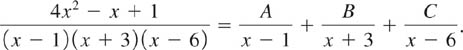
By following the same steps as in Example 1, we would find that the analogue of (7) is now three equations in the three unknowns A, B, and C. The point is this: the more linear factors in the denominator, the larger the system of equations we must solve. There is an algebraic procedure worth learning that can cut down on some of the algebra. To illustrate, let’s return to the identity (5). Since the equality is true for every value of x, it holds for x = 1 and x = −3, the zeros of the denominator. Setting x = 1 in (5) gives 3 = 4A, from which it follows immediately that ![]() . Similarly, by setting x = − 3 in (5), we obtain −5 = (−4)B or
. Similarly, by setting x = − 3 in (5), we obtain −5 = (−4)B or ![]() .
.
CASE 2: Q(x) Contains Repeated Linear Factors
If the denominator Q(x) contains a repeated linear factor (ax + b)n, n > 1,then unique real constants C1, C2,…, Cn can be found such that the partial fraction decomposition of P(x)/Q(x) contains the terms
![]()
EXAMPLE 2 Repeated Linear Factors
To decompose ![]() into partial fractions, we first observe that the denominator consists of the repeated linear factor x and the nonrepeated linear factor 2x −1. Based on the forms in (3) and (8), we assume that
into partial fractions, we first observe that the denominator consists of the repeated linear factor x and the nonrepeated linear factor 2x −1. Based on the forms in (3) and (8), we assume that
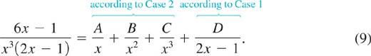
Multiplying (9) by x3(2x − 1) clears it of fractions and yields
![]()
![]()
Now the zeros of the denominator in the original expression are x = 0 and ![]() . If we then set x = 0 and
. If we then set x = 0 and ![]() in (10), we find, in turn, that C = 1 and D = 16. Because the denominator of the original expression has only two distinct zeros, we can find A and B by equating the corresponding coefficients of x3 and x2 in (11):
in (10), we find, in turn, that C = 1 and D = 16. Because the denominator of the original expression has only two distinct zeros, we can find A and B by equating the corresponding coefficients of x3 and x2 in (11):
![]()
![]() The coefficients of x3 and x2 on the left-hand side of (11) are both 0.
The coefficients of x3 and x2 on the left-hand side of (11) are both 0.
Using the known value of D, the first equation yields A = −D/2 = −8. The second then gives B = A/2 = −4. The partial fraction decomposition is
![]()
![]()
CASE 3: Q(x) Contains Nonrepeated Irreducible Quadratic Factors
If the denominator Q(x) contains nonrepeated irreducible quadratic factors aix2 + bix + ci, then unique real constants A1, A2,…, An, B1, B2,…, Bn can be found such that the partial fraction decomposition of P(x)/Q(x) contains the terms
![]()
EXAMPLE 3 Irreducible Quadratic Factors
To decompose ![]() into partial fractions, we first observe that the quadratic polynomials x2 = 1 and x2 + 2x + 3 are irreducible over the real numbers. Hence by (12) we assume that
into partial fractions, we first observe that the quadratic polynomials x2 = 1 and x2 + 2x + 3 are irreducible over the real numbers. Hence by (12) we assume that
![]()
![]() Use the quadratic formula. For either factor you will find that b2 − 4ac = 0.
Use the quadratic formula. For either factor you will find that b2 − 4ac = 0.
After clearing fractions in the preceding line, we find
![]()
Because the denominator of the original fraction has no real zeros, we have no recourse except to form a system of equations by comparing coefficients of all powers of x:
Using C = −A and D = −3B from the first and fourth equations, we can eliminate C and D in the second and third equations:
![]()
Solving this simpler system of equations yields A = 1 and B = 1. Hence, C = −1 and D = − 3. The partial fraction decomposition is
![]()
![]()
CASE 4: Q(x) Contains Repeated Irreducible Quadratic Factors
If the denominator Q(x) contains a repeated irreducible quadratic factor (ax2 + bx + c)n, n = 1, then unique real constants A1, A2,…, An, B1, B2,…, Bn can be found such that the partial fraction decomposition of P(x)/Q(x) contains the terms
![]()
EXAMPLE 4 Repeated Quadratic Factor
Decompose ![]() into partial fractions.
into partial fractions.
Solution The denominator contains only the repeated irreducible quadratic factor x2 = 4. As indicated in (13), we assume a decomposition of the form
![]()
Clearing fractions by multiplying both sides of the preceding equality by (x2 + 4)2 gives
![]()
As in Example 3, the denominator of the original has no real zeros, and so we must solve a system of four equations for A, B, C, and D. To that end we rewrite (14) as
![]()
and compare coefficients of like powers (match the colors) to obtain

From this system we find that A = 0, B = 1, C = 0, and D = −4. The required partial fraction decomposition is then
![]()
![]()
EXAMPLE 5 Combination of Cases
Determine the form of the decomposition of ![]()
Solution The denominator contains a single linear factor x − 5, a repeated linear factor x = 2, and a repeated irreducible quadratic factor x2 = 1. By Cases 1, 2, and 4 the assumed form of the partial fraction decomposition is
![]()
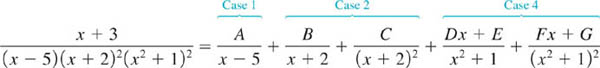
NOTES FROM THE CLASSROOM
We assumed throughout the foregoing discussion that the degree of the numerator P(x) was less than the degree of the denominator Q(x). If, however, the degree of P(x) is greater than or equal to the degree of Q(x), then P (x)/Q(x) is an improper fraction. We can still do partial fraction decomposition, but the process starts with long division until a polynomial quotient and a proper fraction is attained. For example, long division gives
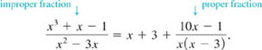

Then by using Case 1 we finish the problem with the decomposition of the proper-fraction term in the last equality:
![]()
See Problems 25–30 in Exercises 3.6.
3.6 Exercises
Answers to selected odd-numbered problems begin on page ANS–11.
In Problems 1–24, find the partial fraction decomposition of the given rational expression.
1. ![]()
2. ![]()
3. ![]()
4. ![]()
5. ![]()
6. ![]()
7. ![]()
8. ![]()
9. ![]()
10. ![]()
11. ![]()
12. ![]()
13. ![]()
14. ![]()
15. ![]()
16. ![]()
17. ![]()
18. ![]()
19. ![]()
20. ![]()
21. ![]()
22. ![]()
23. ![]()
24. ![]()
In Problems 25–30, first use long division followed by partial fraction decomposition.
25. ![]()
26. ![]()
27. ![]()
28. ![]()
29. ![]()
30. ![]()
3.7 The Area Problem

![]() Introduction As we saw in Section 2.9, the fundamental motivating problem of differential calculus, Find a tangent line to the graph of a function f, is answered by the notion of the derivative of the function. Differential calculus is the study of the properties and applications of the derivative of a function y = f(x). Integral calculus, on the other hand, is the study of the properties and the applications of the definite integral of a function y = f(x). As mentioned in Section 2.9, the historical problem that leads to the concept of the definite integral is, Find the area under the graph of a function f. We examine the area problem in this section.
Introduction As we saw in Section 2.9, the fundamental motivating problem of differential calculus, Find a tangent line to the graph of a function f, is answered by the notion of the derivative of the function. Differential calculus is the study of the properties and applications of the derivative of a function y = f(x). Integral calculus, on the other hand, is the study of the properties and the applications of the definite integral of a function y = f(x). As mentioned in Section 2.9, the historical problem that leads to the concept of the definite integral is, Find the area under the graph of a function f. We examine the area problem in this section.
![]() Area Under a Graph Throughout the discussion that follows we will assume that y = f(x) is a function that is continuous and nonnegative on an interval [a, b]. Recall that the concept of continuity has been mentioned several times in previous sections; in this case, the graph of f has no breaks, gaps, or holes in it anywhere on the interval [a, b]. The requirement that f be nonnegative, that is, f(x) ≥ 0 for all x in [a, b], means that no portion of its graph on the interval is below the x-axis. Specifically, then,
Area Under a Graph Throughout the discussion that follows we will assume that y = f(x) is a function that is continuous and nonnegative on an interval [a, b]. Recall that the concept of continuity has been mentioned several times in previous sections; in this case, the graph of f has no breaks, gaps, or holes in it anywhere on the interval [a, b]. The requirement that f be nonnegative, that is, f(x) ≥ 0 for all x in [a, b], means that no portion of its graph on the interval is below the x-axis. Specifically, then,
By the area under a graph we mean the area A of the region in the plane bounded by the graph of f, the lines x = a and x = b, and the x-axis.
See FIGURE 3.7.1.
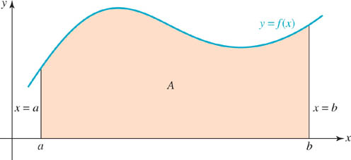
FIGURE 3.7.1 Area A under a graph
To get to the answer of the question, What is the exact value of A? we begin with a method for systematically approximating A. The basic idea is simply this: build rectangles across the interval [a, b] and use the sum of the areas of the rectangles as an approximation for A.
![]() Approximating the Area One possible systematic procedure for approximating the value of the area A under a graph is summarized next.
Approximating the Area One possible systematic procedure for approximating the value of the area A under a graph is summarized next.
(i) Subdivide the interval [a, b] into n subintervals [xk−1, xk], where
![]()
so that each subinterval has the same width ![]() . This is called a regular partition of the interval [a, b].
. This is called a regular partition of the interval [a, b].
(ii) Choose a number x*k in each of the n subintervals [xk−1, xk] and form the n products f(xk*) ∆x. Since the area of a rectangle is length × width, f(xk*) ∆x is the area of the rectangle of length f(xk*) and width ∆x built up on the kth subinterval [xk−1, xk] The n numbers x1*, x2*, x3*,…, xn* are called sample points. See FIGURE 3.7.2.
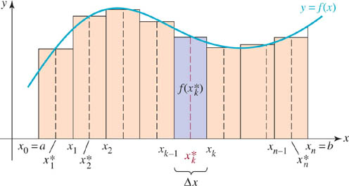
FIGURE 3.7.2 n rectangles of width ∆x and length ![]()
(iii) The sum of the areas of the n rectangles represents an approximation to the value of the area,
![]()
To simplify the hand calculations, the sample points ![]() ,k= 1, 2, …, are generally chosen to be either the left-hand endpoint or the right-hand endpoint of each subinterval [xk−1, xk]
,k= 1, 2, …, are generally chosen to be either the left-hand endpoint or the right-hand endpoint of each subinterval [xk−1, xk]
EXAMPLE 1 Area of a Triangular Region
Approximate the area A under the graph of f(x) = x on the interval [0, 1] using four subintervals of equal width and choosing
(a) ![]() as the left-hand endpoint of each subinterval, and
as the left-hand endpoint of each subinterval, and
(b) ![]() as the right-hand endpoint of each subinterval.
as the right-hand endpoint of each subinterval.
See FIGURE 3.7.3.
Solution By dividing [0, 1] into four subintervals, the width of each subinterval is ![]()
(a) If ![]() is the left-hand endpoint of each of the four subintervals, then
is the left-hand endpoint of each of the four subintervals, then ![]() and
and ![]() . See FIGURE 3.7.4(a). We have from (1),
. See FIGURE 3.7.4(a). We have from (1),
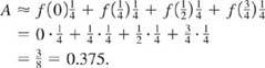
(b) If ![]() is the right-hand endpoint of each of the four subintervals, then
is the right-hand endpoint of each of the four subintervals, then ![]()
See Figure 3.7.4(b). We have from (1),
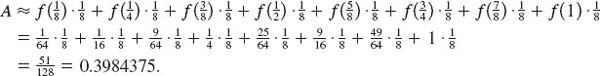
![]()
As can be seen in Figures 3.7.4(a) and 3.7.4(b), the value obtained in part (a) of Example 1 underestimates the area A, whereas the value in part (b) overestimates A, that is, 0.375 < A < 0.625. We can compare these approximations with the actual area. Since the area under the graph of f(x) = x on the interval [0, 1 ] is the area of a right triangle of base = 1 and height = 1, the exact area is ![]() .
.
There is no special reason that we chose the sample points ![]() , k = 1, 2,…, n, to be the left-hand and then the right-hand endpoints of the subintervals [xk−1, xk], other than convenience. We could pick
, k = 1, 2,…, n, to be the left-hand and then the right-hand endpoints of the subintervals [xk−1, xk], other than convenience. We could pick ![]() randomly in each subinterval. In Problem 3 of Exercises 3.7 you are asked to approximate the area in Example 1 using the midpoint of each subinterval.
randomly in each subinterval. In Problem 3 of Exercises 3.7 you are asked to approximate the area in Example 1 using the midpoint of each subinterval.
Intuitively, the more rectangles we use the better (1) approximates the area A under a graph. The trade-off, of course, is that we must do more calculations.
EXAMPLE 2 Area Under a Parabola
Approximate the area A under the graph of f(x) = x2 on the interval [0, 1] using eight subintervals of equal width and choosing
(a) ![]() as the left-hand endpoint of each subinterval, and
as the left-hand endpoint of each subinterval, and
(b) ![]() as the right-hand endpoint of each subinterval.
as the right-hand endpoint of each subinterval.
See FIGURE 3.7.5.
Solution By dividing [0, 1] into eight subintervals, the width of each subinterval
is ![]() .
.
(a) If ![]() is the left-hand endpoint of each of the four subintervals, then
is the left-hand endpoint of each of the four subintervals, then
![]()
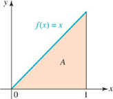
FIGURE 3.7.3 Area A in Example 1
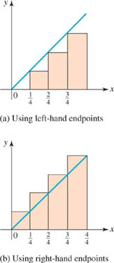
FIGURE 3.7.4 Approximating the area A in Example 1
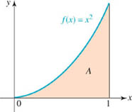
FIGURE 3.7.5 Area A in Example 2
See FIGURE 3.7.6(a). We have from (1),
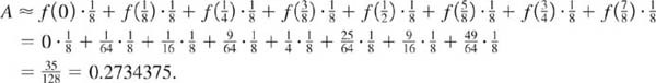
(b) If ![]() is the right-hand endpoint of each of the four subintervals, then
is the right-hand endpoint of each of the four subintervals, then
![]()
See Figure 3.7.6(b). We have from (1),
![]()
From Figure 3.7.6(a) we see that the area of the seven rectangles underestimates A in Example 2, whereas the eight rectangles in Figure 3.7.6(b) overestimates A. From the calculations in Example 2 we can write 0.2734375 < A < 0.3984375. But an observation is in order at this point. Don’t assume that by using left-hand endpoints followed by the right-hand endpoints of the subintervals for ![]() that we always get, in turn, a lower estimate followed by an upper estimate of the area A under the graph of f on [a, b]. This occurred in Examples 1 and 2 simply because, in both cases, the function f was increasing on the interval [0, 1].
that we always get, in turn, a lower estimate followed by an upper estimate of the area A under the graph of f on [a, b]. This occurred in Examples 1 and 2 simply because, in both cases, the function f was increasing on the interval [0, 1].
![]() Summation Notation Writing out sums such as (1) can become very tedious. To facilitate the discussion of the area problem, a special notation for summation is used in calculus. Suppose ak denotes a real number that depends on an integer k. The sum of n such real numbers ak, a1 + a2 + a3 + …. an, is denoted by the symbol
Summation Notation Writing out sums such as (1) can become very tedious. To facilitate the discussion of the area problem, a special notation for summation is used in calculus. Suppose ak denotes a real number that depends on an integer k. The sum of n such real numbers ak, a1 + a2 + a3 + …. an, is denoted by the symbol ![]() , that is,
, that is,
![]()
Since Σ is the capital Greek letter sigma, (2) is called summation notation or sigma notation. The integer k is called the index of summation and takes on consecutive integer values starting with k = 1 and ending with k = n. For example, the sum of the first 100 squared positive integers,
![]()
can be written compactly as
Using sigma notation, the sum of the areas in (1) can be written as
![]()
FIGURE 3.7.6 Approximating the area A in Example 2
![]() Area It should seem believable that we can reduce the error inherent in the method of approximating an area A under a graph by summing areas of rectangles by using more and more rectangles (n → ∞) of decreasing width
Area It should seem believable that we can reduce the error inherent in the method of approximating an area A under a graph by summing areas of rectangles by using more and more rectangles (n → ∞) of decreasing width ![]() . Thus the 32 rectangles in FIGURE 3.7.7 should give us a better approximation to area A in Figure 3.7.1 than the eight rectangles shown in Figure 3.7.2. Indeed that is the case. It can be proved that when f is continuous on [a, b] and f(x) ≥ 0 for all x in the interval, the area A under the graph of the function y = f(x) on the interval is given by the limit
. Thus the 32 rectangles in FIGURE 3.7.7 should give us a better approximation to area A in Figure 3.7.1 than the eight rectangles shown in Figure 3.7.2. Indeed that is the case. It can be proved that when f is continuous on [a, b] and f(x) ≥ 0 for all x in the interval, the area A under the graph of the function y = f(x) on the interval is given by the limit
![]()
FIGURE 3.7.7 Using more rectangles improves the approximation to area A
The limit (3) exists regardless of how the sample points ![]() are chosen in the subintervals [x0, x1], [x1, x2], [x2, x3],…, [xn−1, xn] Thus in (3), each sample point
are chosen in the subintervals [x0, x1], [x1, x2], [x2, x3],…, [xn−1, xn] Thus in (3), each sample point ![]() could always be chosen, say, to be the right-hand endpoint of each subinterval. Since we are in no position to deal, in general terms, with limits of the kind given in (3), we leave that aspect of the area problem to a course in calculus. But if you are willing to put in the time to work Problems 15–22, then Problems 23 and 24 will give you a small taste of what is involved in computing area A by the limiting process given in (3).
could always be chosen, say, to be the right-hand endpoint of each subinterval. Since we are in no position to deal, in general terms, with limits of the kind given in (3), we leave that aspect of the area problem to a course in calculus. But if you are willing to put in the time to work Problems 15–22, then Problems 23 and 24 will give you a small taste of what is involved in computing area A by the limiting process given in (3).
We said at the start that the area problem is the motivating problem for the definite integral. You ask: So what is a definite integral? It is now just a small jump from (3) to the concept of the definite integral.
DEFINITE INTERVAL
Let the function f be continuous on [a, b] The definite integral of f from x = a to x = b, denoted by,f(x) is
The integral symbol ∫ in (4), as used by Wilhelm Gottfried Leibniz (1646–1716) (who is considered the co-inventor of calculus, along with Isaac Newton (1643–1727)), is simply an elongated S for the word “sum.”
NOTES FROM THE CLASSROOM
(i) If read quickly, you might conclude that formula (4) is the same as (3). In a way this is correct; however, (4) is a more general concept (notice that we are not requiring f to be nonnegative on the interval [a, b]). Thus, a definite integral need not be area. Also, in its most general setting, even the conditions of continuity of f and the use of a regular partition are dropped in the definition of the definite integral. What, then, is a definite integral? For now, accept the fact that a definite integral is simply a real number that can be negative, zero, or positive. When the conditions of continuity and nonnegativity are imposed on y = f(x) on the interval [a, b], then the area under the graph is ![]() . Also, you should be aware that the interpretations of derivative and the definite integral are much broader than just slopes of tangent lines and areas under graphs. As you progress through courses in mathematics, sciences, and engineering you will see many diverse applications of the derivative and the definite integral.
. Also, you should be aware that the interpretations of derivative and the definite integral are much broader than just slopes of tangent lines and areas under graphs. As you progress through courses in mathematics, sciences, and engineering you will see many diverse applications of the derivative and the definite integral.

(ii) In this chapter we worked principally with polynomial functions. Polynomial functions are the fundamental building blocks of a class known as algebraic functions. In Section 3.5 we saw that a rational function is the quotient of two polynomial functions. In general, an algebraic function f involves a finite number of additions, subtractions, multiplications, divisions, and roots of polynomial functions. Thus
![]()
are algebraic functions. Indeed, all the functions in Chapters 2 and 3 are algebraic functions. Starting with the next chapter we consider functions that belong to a different class known as transcendental functions. A transcendental function f is defined to be one that is not algebraic. The six trigonometric functions (Chapter 4) and the exponential and logarithmic functions (Chapter 5) are examples of transcendental functions.
3.7 Exercises
Answers to selected odd-numbered problems begin on page ANS–11.
In Problems 1–4, the function f and the interval are given in Example 1.
1. Approximate the area A, this time using eight subintervals of equal width and choosing x*k as the left-hand endpoint of each subinterval. Draw the eight rectangles.
2. Approximate the area A, this time using eight subintervals of equal width and choosing x*k as the right-hand endpoint of each subinterval. Draw the eight rectangles.
3. Approximate the area A, this time using four subintervals of equal width but choosing x*k as the midpoint of each subinterval. Draw the four rectangles.
4. Compare the approximation obtained in Problem 3 of the exact area A = 0.5. Explain why your answer in Problem 3 is not surprising.
5. Approximate the area under the graph of f (x) = x + 2 on the interval [−1, 2] using six subintervals of equal width and choosing:
(a) x*k as the left-hand endpoint of each subinterval, and
(b) x*k as the right-hand endpoint of each subinterval.
6. Repeat Problem 5 using twelve subintervals of equal width.
7. Approximate the area under the graph of f (x) = −x2 + 5x on the interval [0, 5] using five subintervals of equal width and choosing:
(a) x*k as the left-hand endpoint of each subinterval, and
(b) x*k as the right-hand endpoint of each subinterval.
8. Repeat Problem 7 using ten subintervals of equal width.
9. Approximate the area under the graph of f(x) = −x2 +5 x on the interval [0, 5] using five subintervals of equal width and choosing x*k as the midpoints of each subinterval.
10. Approximate the area under the graph of f(x) = −x3 + 2x2 on the interval [0, 2] using ten subintervals of equal width and choosing x*k as the right-hand endpoint of each subinterval.
11. Find two different approximations for the area A under the graph y = f(x) on the interval [1, 4] shown in FIGURE 3.7.8.
12. Find two different approximations for the area A under the graph y = f(x) on the interval shown in FIGURE 3.7.9.
Miscellaneous Applications
13. Lakefront Property Suppose a realtor wants to find the area of an irregularly shaped piece of land that is bounded between a 1 mile-long segment of a straight road and the shore of a lake. Measurements (in feet) of the perpendicular distances from the road to the lake are taken at equally spaced intervals along the road as shown in FIGURE 3.7.10. Find two different approximations of the area of the land. Express your answer in acres using the fact that 1 acre = 43,560 ft2.
14. For the Fish The large irregularly shaped fish pond shown in FIGURE 3.7.11 is filled with water to a uniform depth of 4 ft. Find an approximation to the number of gallons of water in the pond. Measurements are in feet and the vertical spacing between the horizontal measurements is 1.86 ft. There are 7.48 gallons in 1 cubic foot of water. [Hint: The volume of water is the area of the surface × depth.]
For Discussion
If c denotes a constant—that is, independent of the summation index k—then Σnk+1 c means c + c + c + … + c. Since there are n c’s in this sum, we have
![]()
In Problems 15 and 16, use (5) to find the numerical value of the given sum.
15. ![]()
16. ![]()
The sum of the first n positive integers can be written Σnk+1 k. If this sum is denoted by S, then
![]()
FIGURE 3.7.8 Graph for Problem 11
FIGURE 3.7.9 Graph for Problem 12
FIGURE 3.7.10 Land in Problem 13
FIGURE 3.7.11 Fish pond in Problem 14
can also be written as
![]()
If we add (6) and (7), then

Solving for S gives ![]() , or
, or
![]()
In Problems 17 and 18, use (8) to find the numerical value of the given sum.
17. ![]()
18. ![]()
Here are two properties of summation notation:
![]()
![]()
In Problems 19–22, use (5) and (8)–(10) to find the numerical value of the given sum.
19. ![]()
20. ![]()
21. ![]()
22. ![]()
In Problems 23 and 24, use the results in (5) and (8)–(10) and the limit definition of area given in (3) to find the exact value of the area A. In each case, partition the given interval into n subintervals of width ∆x = (b − a)/n and use xk* as the right-hand end-point of each subinterval.
23. A is the area under the graph of f(x) = 2x + 1 on the interval [0, 4]
24. A is the area under the graph of f(x) = − 3x + 12 on the interval [1, 3]
25. Consider the trapezoid given in FIGURE 3.7.12.
(a) Discuss how the area A can be approximated using (1) of this section.
(b) Using well-known area formulas, find a formula that expresses A in terms of h1, h2, and b.
CHAPTER 3 Exercises
Answers to selected odd-numbered problems begin on page ANS–12.
In Problems 1–16, fill in the blanks.
1. The graph of the polynomial function f(x) = x3(x − 1)2(x − 5) is tangent to the x-axis at______and passes through the x-axis at______.
2. A third-degree polynomial function with zeros 1 and 3i is______.
FIGURE 3.7.12 Trapezoid in Problem 25
3. The end behavior of the graph of f(x) = x2(x + 3)(x − 5) resembles the graph of the power function f(x) =______.
4. The polynomial function f(x) = x4 − 3x3 + 17x2 − 2x + 2 has______(how many) possible rational zeros.
5. For f(x) = kx2(x − 2)(x − 3), f(−1) + 8 if k =______.
6. The y-intercept of the graph of the rational function ![]() is______.
is______.
7. The vertical asymptotes for the graph of the rational function ![]() are______.
are______.
8. The x-intercepts of the graph of the rational function ![]() are______.
are______.
9. The horizontal asymptote for the graph of the rational function ![]() is______.
is______.
10. A rational function whose graph has the horizontal asymptote y = 1 and x-intercept (3, 0) is______.
11. The graph of the rational function ![]() , where n is a nonnegative integer, has the horizontal asymptote y = 0 when n =______.
, where n is a nonnegative integer, has the horizontal asymptote y = 0 when n =______.
12. The graph of the polynomial function f(x) = 3x5 − 4x2 = 5x − 2 has at most ______ turning points.
13. If i is a zero of
![]()
then three other zeros are______.
14. The rational function ![]() has______(how many) asymptotes.
has______(how many) asymptotes.
15. Suppose that when a polynomial function f of degree 5 is divided by x − 3 we get
![]()
The degree of the quotient q(x) is______.
16. If f is the polynomial function in Problem 15, then f(3) =______.
In Problems 17–34, answer true or false.
17. f(x) = 2x3 − 8x−2 + 5 is not a polynomial.______
18. ![]() is a rational function.______
is a rational function.______
19. The graph of a polynomial function can have no holes in it.______
20. A polynomial function of degree 4 has exactly four real zeros.______
21. When a polynomial of degree greater than one is divided by x − 1, the remainder is always a constant.______
22. If the coefficients a, b, c, and d of the polynomial function f(x) = ax3 + bx2 + cx + d are positive integers, thenf has no positive real zeros.______
23. The polynomial equation 2x7 + 1 −x has a solution in the interval [0, 1].______
24. The graph of the rational function f(x) = (x2 + 1)/x has a slant asymptote.______
25. The graph of the polynomial function f(x) = 4x6 + 3x2 is symmetric with respect to the y-axis.______
26. The graph of a polynomial function that is an odd function must pass through the origin.______
27. An asymptote is a line that the graph of a function approaches but never crosses.______
28. The point ![]() is on the graph of
is on the graph of ![]() .______
.______
29. The graph of a rational function f(x) = P(x)/Q(x) has a slant asymptote when the degree of P is greater than the degree of Q.______
30. If 3 − 4i is a zero of a polynomial function f(x) with real coefficients, then 3 = 4i is also a zero of f(x).______
31. A polynomial function must have at least one rational zero.______
32. The graph of f(x) = x4 + 5 x2 + 2 does not cross the x-axis.______
33. If (−1, 6) and (4, − 2) are two points on the graph of a polynomial function f, then f has at least one zero in the open interval (−1, 4).______
34. If the end behavior of a polynomial function f is that its graph goes up for large values of |x|, then the degree of f must be an even positive integer.______
In Problems 35 and 36, use long division to divide f(x) by d(x).
35. f(x) = 6x5 − 4x3 + 2x2 + 4, d(x) + 2x2 − 1
36. f(x) = 15x4 − 2x3 + 8x + 6, d(x) = 5x3 + x + 2
In Problems 37 and 38, use synthetic division to divide f(x) by d(x).
37. f(x) = 7x4 − 6x2 + 9x + 3, d(x) = x − 2
38. f(x) = 4x3 + 7x2 − 8x, d(x) = x + 1
39. Without actually performing the division, determine the remainder when f(x) = 5x3 − 4x2 + 6x − 9 is divided by d(x) = x + 3.
40. Use synthetic division and the Remainder Theorem to find f(c) for
![]()
when c = 2.
41. Determine the values of the positive integer n such that f(x) = xn + cn is divisible by d(x) = x + c.
42. Suppose that
![]()
is divided by d(x) = x − 1. What is the remainder?
43. List, but do not test, all possible rational zeros of
![]()
44. Find the complete factorization of f(x) = 12x3 + 16x2 + 7x + 1.
In Problems 45 and 46, verify that each of the indicated numbers is a zero of the given polynomial function f(x). Find all other zeros and then give the complete factorization of f(x).
45. 2; f(x) = (x − 3)3 + 1
46. −1; f(x) = (x + 2)4 − 1
In Problems 47–50, find the real value of k so that the given condition is satisfied.
47. the remainder in the division of f(x) = x4 − 3x3 −x2 + kx − 1 by g(x) = x − 4 is r + 5
48. ![]() is a factor of f(x) = 8x2 − 4kx + 9
is a factor of f(x) = 8x2 − 4kx + 9
49. x −k is a factor of f(x) = 2x3 + x2 + 2x − 12
50. the graph of ![]() has a hole at x = k
has a hole at x = k
In Problems 51–54, find the partial fraction decomposition of the given rational expression.
51. ![]()
52. ![]()
53. ![]()
54. ![]()
In Problems 55 and 56, find a polynomial function f of indicated degree whose graph is given in the figure.
55. fifth degree
56. sixth degree
FIGURE 3.R.1 Graph for Problem 55
FIGURE 3.R.2 Graph for Problem 56
In Problems 57 and 58, find a rational function f whose graph is given in the figure.
57.
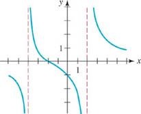
FIGURE 3.R.3 Graph for Problem 57
58.
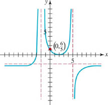
FIGURE 3.R.4 Graph for Problem 58
In Problems 59–68, match the given rational function with one of the graphs (a)–(j).
(a) 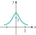
FIGURE 3.R.5
(b) 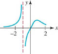
FIGURE 3.R.6
(c) 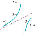
FIGURE 3.R.7
(d) 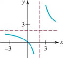
FIGURE 3.R.8
(e) 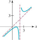
FIGURE 3.R.9
(f) 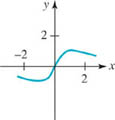
FIGURE 3.R.10
(g) 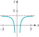
FIGURE 3.R.11
(h) 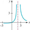
FIGURE 3.R.12
(i) 
FIGURE 3.R.13
(j) 
FIGURE 3.R.14
59. ![]()
60. ![]()
61. ![]()
62. ![]()
63. ![]()
64. ![]()
65. ![]()
66. ![]()
67. ![]()
68. ![]()
In Problems 69 and 70, find the asymptotes for the graph of the given rational function. Find x- and y-intercepts of the graph. Sketch the graph of f
69. ![]()
70. ![]()