5 Exponential and Logarithmic Functions

Chapter Outline

5.1 Exponential Functions

5.2 Logarithmic Functions

5.3 Exponential and Logarithmic Models

5.4 The Hyperbolic Functions

       Chapter 5 Review Exercises

5.1 Exponential Functions

Introduction In the preceding chapters we considered functions such as f(x) = x², that is, a function with a variable base x and constant power or exponent 2. We now examine functions such as f(x) = 2^x having a constant base 2 and a variable exponent x.

The domain of an exponential f defined in (1) is the set of all real numbers (−∞, ∞).

In (1) the base b is restricted to positive numbers in order to guarantee that b^x is always a real number. For example, with this restriction we avoid complex numbers such as (−4)^1/2. Also, the base b = 1 is of little interest to us since (1) is the constant function f(x) = 1^x = 1.

Exponents As just mentioned, the domain of an exponential function (1) is the set of all real numbers. This means that the exponent x can be either a rational or an irrational number. For example, if the base is b = 3 and the exponent x is a rational number—for example, and x = 1.4—then

For an exponent x that is an irrational number, b^x is defined, but its precise definition is beyond the scope of this text. We can, however, suggest a procedure for defining a number such as . From the decimal representation we see that the rational numbers

are successively better approximations to . By using these rational numbers as exponents, we would expect that the numbers

are then successively better approximations to . In fact, this can be shown to be true with a precise definition of b^x for an irrational value of x. But on a practical level, we can use the key on a calculator to obtain the approximation 4.728804388 to .

Laws of Exponents In most algebra texts the laws of exponents are stated first for integer exponents and then for rational exponents. Since b^x can be defined for all real numbers x when b > 0, it can be proved that these same laws of exponents hold for all real-number exponents. If a > 0, b > 0, and x, x₁, and x₂ denote real numbers, then

 (i) b^x₁. b^x₂ = b^{x₁ + x₂}

(ii)

(iii)

(iv) (b^x₁)^x₂ = b^x₁x₂

(v) (ab)^x = a^xb^x

(vi)

EXAMPLE 1 Rewriting a Function

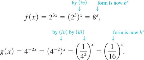
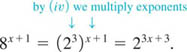
At times, we will use the laws of exponents to rewrite a function in a different form. For example, neither f(x) = 2^3x nor g(x) = 4^−2x has the precise form of the exponential function defined in (1). However, by the laws of exponents f can be rewritten as f(x) = 8^x (b = 8 in (1)), and g can be recast as . The details are shown below:

Graphs We distinguish two types of graphs for (1) depending on whether the base b satisfies b > 1 or 0 < b < 1. The next two examples illustrate, in turn, the graphs of f(x) = 3^x and Before graphing, we can make some intuitive observations about both functions. Since the bases b = 3 and are positive, the values of 3^x and are positive for every real number x. Moreover, neither 3^x nor can be zero for any x and so the graphs of f(x) = 3^xand have no x-intercepts. Also, 3° = 1 and , and so f (0) = 1 in each case. This means that the graphs of f(x) = 3^x and have the same y-intercept (0, 1).

EXAMPLE 2 Graph for b > 1

Graph the function f(x) = 3^x.

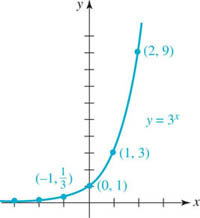
FIGURE 5.1.1 Graph of function in Example 2

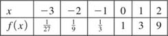
Solution We first construct a table of some function values corresponding to preselected values of x. As shown in FIGURE 5.1.1, we plot the corresponding points obtained from the table and connect them with a continuous curve. The graph shows that f is an increasing function on the interval (−∞, ∞).

EXAMPLE 3 Graph for 0 < b < 1

Graph the function .

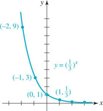
FIGURE 5.1.2 Graph of function in Example 3

Solution Proceeding as in Example 2, we construct a table of some function values corresponding to preselected values of x. Note, for example, by the laws of exponents

As shown in FIGURE 5.1.2, we plot the corresponding points obtained from the table and connect them with a continuous curve. In this case the graph shows that f is a decreasing function on the interval (− ∞, ∞).

Exponential functions with bases satisfying 0 < b < 1, such as , are frequently written in an alternative manner. We note that is the same as y = 3^−x. From this last result we see that the graph of y = 3^−x is simply the graph of y = 3^x reflected in the y-axis.

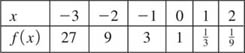
Horizontal Asymptote FIGURE 5.1.3 illustrates the two general shapes that the graph of an exponential function f(x) = b^x can have. There is, however, one more important aspect of all such graphs. Observe in Figure 5.1.3 that for b > 1,

whereas for 0 < b < 1,

In other words, the line y = 0 (the x-axis) is a horizontal asymptote for both types of exponential graphs.

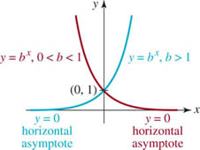
FIGURE 5.1.3 fincreasing for b > 1; f decreasing for 0 < b < 1

Properties of an Exponential Function The following list summarizes some of the important properties of the exponential function f with base b. Reexamine the graphs in Figures 5.1.1–5.1.3 as you read this list.

• The domain of f is the set of real numbers, that is, (− ∞, ∞).
• The range of f is the set of positive real numbers, that is, (0, ∞).
• The y-intercept of f is (0, 1). The graph of f has no x-intercept.
• The function f is increasing for b > 1 and decreasing for 0 < b < 1. (2)
• The x-axis, that is, y = 0, is a horizontal asymptote for the graph of f.
• The function f is continuous on (− ∞, ∞).
• The function f is one-to-one.

Although the graphs y = b^x in the case, say, when b > 1, all share the same basic shape and all pass through the same point (0, 1), there are subtle differences. The larger the base b the more steeply the graph rises as x increases. In FIGURE 5.1.4 we compare the graphs of y = 5^x, y = 3^x, y = 2^x, and y = (1.2)^x in green, blue, gold, and red, respectively, on the same coordinate axes. We see from its graph that the values of y = (1.2)^x increase slowly as x increases. For example, for y = (1.2)^x, f (3) = (1.2)³ = 1.728, whereas for y = 5^x, f (3) = 5³ = 125.

FIGURE 5.1.4 Graphs of y = b^x for b = 1.2, 2, 3, 5

The fact that (1) is a one-to-one function follows from the horizontal line test discussed in Section 2.7. Note in Figures 5.1.1–5.1.4 a horizontal line can cross or intersect an exponential graph in at most one point.

Of course, we can obtain other kinds of graphs by rigid and nonrigid transformations, or when an exponential function is combined with other functions by either an arithmetic operation or by function composition. In the next several examples we examine variations of the exponential graph.

For reflections in a coordinate axis, see (ii) on page 62 of Section 2.2

EXAMPLE 4 Horizontally Shifted Graph

Graph the function f(x) = 3^x+2.

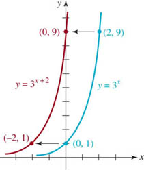
FIGURE 5.1.5 Shifted graph in Example 4

Solution From the discussion in Section 2.2 you should recognize that the graph of f(x) = 3^x+2 is the graph of y = 3^x shifted 2 units to the left. Recall that since the shift is a rigid transformation to the left, the points on the graph of f(x) = 3^{x + 2} are the points on the graph of y = 3^x moved horizontally 2 units to the left. This means that the y-coordinates of points (x, y) on the graph of y = 3^x remain unchanged, but 2 is subtracted from all the x-coordinates of the points. Thus we see from FIGURE 5.1.5 that the points (0, 1) and (2, 9) on the graph of y = 3^x are moved, in turn, to the points (−2, 1) and (0, 9) on the graph of f(x) = 3^x+2.

The function f(x) = 3^x+2 in Example 4 can be rewritten, if desired, as f(x) = 9 · 3^x. By (i) of the laws of exponents, 3^x+2 = 3²3^x = 9 • 3^x. In this manner we can reinterpret the graph of f(x) = 3^x+2 as a vertical stretch of the graph of y = 3^x by a factor of 9. For example, (1, 3) is on the graph of y = 3^x, whereas, (1, 9 • 3) = (1, 27) is on the graph of f(x) = 3^x+2.

The Number e Almost every student of mathematics has heard of, and has likely worked with, the famous irrational number π = 3.141592654.… Recall that an irrational number is a nonrepeating and nonterminating decimal. In calculus and applied mathematics the irrational number

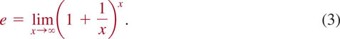
arguably plays a role more important than the number π. The usual definition of the number e is the number that the function f(x) = (1 + 1/x)^x approaches as we let x become large without bound in the positive direction, that is, f(x) → e as x → ∞. Using the limit notation introduced in Sections 1.5 and 2.9, we write

See Problems 55 and 57 in Exercises 5.1. You will often see an alternative definition of the number e. If we let h = 1/x in (3), then as x → ∞ we have simultaneously h → 0. Hence an equivalent form of (3) is

See Problems 56 and 58 in Exercises 5.1. Of course, advancing (3) and (4) as definitions of the number e raises the obvious question: Where do these strange limits come from? An unsatisfying partial answer is: Definitions (3) and (4) come from calculus. While we cannot prove in this course that the limits in (3) and (4) exist, we will, however, discuss the origins of e in Section 5.4.

The Natural Exponential Function When the base in (1) is chosen to be b = e, the function

is called the natural exponential function. Since b = e > 1 and b = 1/e < 1, the graphs of y = e^x and y = e^−x (or y = (1/e)^x) are given in FIGURE 5.1.6.

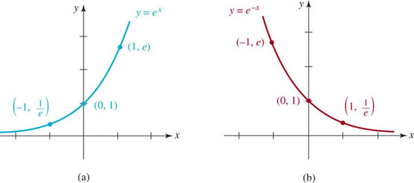
FIGURE 5.1.6 Graphs of the natural exponential function (part (a)) and its reciprocal (part (b))

On the face of it, the exponential function (5) possesses no noticeable graphical characteristic that distinguishes it from, say, the function f(x) = 3^x, and has no special properties other than the ones given in the bulleted list (2). As mentioned, questions as to why (5) is a “natural” and frankly, the most important exponential function, can only be answered fully in courses in calculus and beyond. We will explore some of the importance of the number e in Sections 5.3 and 5.4.

Using rigid transformations, note that the graph of y = e^−x is the graph of f(x) = e^x reflected in the y-axis since y = f (−x) = e^−x. See page 62.

EXAMPLE 5 Vertically Shifted Graph

Graph the function f(x) = 2 − e^−x. State the range.

Solution We first draw the graph of y = e^−x as shown in part (a) of FIGURE 5.1.7. Then we reflect the first graph in the x-axis to obtain the graph of y = − e^−x in part (b) of Figure 5.1.7. Finally, the graph in part (c) of Figure 5.1.7 is obtained by shifting the graph in part (b) upward 2 units.

The y-intercept (0, −1)of y = − e^−x when shifted upward 2 units returns us to the original y-intercept in part (a) of Figure 5.1.7. Finally, the horizontal asymptote y = 0 in parts (a) and (b) of the figure is shifted to y = 2 in part (c) of Figure 5.1.7. From the last graph we can conclude that the range of the function f(x) = 2 − e^−x is the set of real numbers defined by y < 2, that is, the interval (− ∞, 2) on the y-axis.

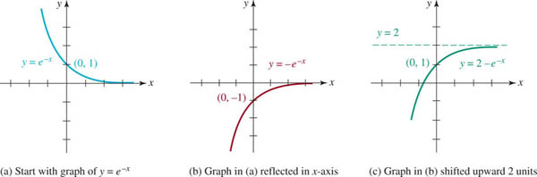
FIGURE 5.1.7 Graph of the function in Example 5

In the next example we graph the function composition of the natural exponential function y = e^x with the simple quadratic polynomial function y = −x².

EXAMPLE 6 A Function Composition

Graph the function .

Solution Because , the y-intercept of the graph is (0, 1). Also, f(x) ≠ 0 since e^−x2 ≠ 0 for every real number x. This means that the graph of f has no x-intercepts. Then from

we conclude that f is an even function, and so its graph is symmetric with respect to the y-axis. Lastly, observe that

By symmetry we can also conclude that f(x) → 0 as x → −∞. This shows that y = 0 is a horizontal asymptote for the graph of f. The graph of f is given in FIGURE 5.1.8.

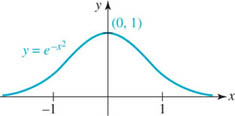
FIGURE 5.1.8 Graph of the function in Example 6

Bell-shaped graphs such as that given in Figure 5.1.8 are very important in the study of probability and statistics.

One-to-One Property Recall from (1) of Section 2.7 that a one-to-one function f possesses the property that if f(x₁ = f(x₂), then x₁ = x₂.Because f(x) = b^x is one-to-one, we have:

As the next example shows, the property in (6) enables us to solve certain kinds of exponential equations.

EXAMPLE 7 An Exponential Equation

Solve 2^x-3 = 8^x+1 for x.

Solution Observe on the right-hand side of the given equality that 8 can be written as a power of 2, that is, 8 = 2³. Furthermore, by the laws of exponents

Thus, the equation is the same as

From the one-to-one property (6) it follows that the exponents are equal, that is, x − 3 = 3x + 3. Solving for x then gives 2x = −6 or x = −3. You are encouraged to check this answer by substituting −3 for x in the original equation.

EXAMPLE 8 An Exponential Equation

Solve 7^{2(x + 1}) = 343 for x.

Solution By noting that 343 = 7³, we have the same base on both sides of the equality:

Thus by (6) we can equate exponents and solve for x:

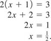
5.1 Exercises
Answers to selected odd-numbered problems begin on page ANS–16.

In Problems 1–12, sketch the graph of the given function f. Find the y-intercept and the horizontal asymptote of the graph. State whether the function is increasing or decreasing.

1.

2.

3. f(x) = −2^x

4. f(x) = −2^−x

5. f(x) = 2^x+1

6^. f(x) = 2^{2 −x}

7. f(x) = −5 + 3^x

8. f(x) = 2 + 3^{2 −x}

9.

10. f(x) = 9 − e^x

11. f(x) = −1 + e^x−3

12. f(x) = −3 − e^x+5

In Problems 13–16, find an exponential function f(x) = b^x such that the graph of f passes through the given point.

13. (3, 216)

14. ( − 1, 5)

15. ( −1, e²)

16. (2, e)

In Problems 17 and 18, determine the range of the given function.

17. f(x) = 5 + e^−x

18. f(x) = 4 − 2^−x

In Problems 19–24, find the x- and y-intercepts of the graph of the given function. Do not graph.

19. f(x) = 2^x − 4

20. f(x) = −3^2x + 9

21. f(x) = xe^x + 10e^x

22. f(x) = x²2^x − 2^x

23. f(x) = x³8^x + 5x²8^x + 6x8^x

24.

In Problems 25–28, use a graph to solve the given inequality.

25. 2^x > 16

26. e^x ≤ 1

27. e^{x −2} < 1

28.

In Problems 29 and 30, use the graph in Figure 5.1.8 to sketch the graph of the given function f.

29.

30.

In Problems 31 and 32, use f (−x) = f(x) to demonstrate that the given function is even. Sketch the graph of f.

31.

32. f(x) = e ^−|x|

In Problems 33–36, use the graphs obtained in Problems 31 and 32 as an aid in sketching the graph of the given function f.

33.

34. f(x) = 2 + 3e^|x|

35. f(x) = − e^{|x −3|}

36.

37. Show that f(x) = 2^x + 2 ^−x is an even function. Sketch the graph of f.

38. Show that f(x) = 2^x − 2 ^−x is an odd function. Sketch the graph of f.

In Problems 39–46, use the one-to-one property (6) to solve the given exponential equation.

39.

40.

41. 8 ^{x − 7} − 1 = 0

42.

43. 2^x · 3^x = 36

44.

45.

46.

In Problems 47–50, either factor or use the quadratic formula to solve the given equation.

47. (5^x)² − 26(5^x) + 25 = 0

48. 64^x − 10(8^x) + 16 = 0

49. 2^x + 2^−x = 2

50. (10^x)² + 10(10^x) − 1000(10^x) − 10,000 = 0

In Problems 51 and 52, find the x-intercept of the graph of the given function.

51. f(x) = e^x+4 − e

52.

In Problems 53 and 54, sketch the graph of the given piecewise-defined function f.

53.

54.

Calculator Problems

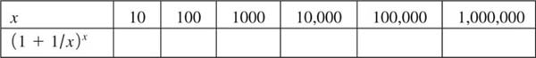
In Problems 55 and 56, use a calculator to fill out the given table.

55.

56.

57. (a) Use a graphing utility to graph the functions f(x) = (1 + 1/x)^xand g(x) = e on the same set of coordinate axes. Use the intervals (0, 10], (0, 100], (0, 1000]. Describe the behavior of f for large values of x. In graphical terms, what is g(x) = e?

(b) Graph the function f in part (a) on the interval [−10, 0). Superimpose that graph with the graph of f on (0, 10] obtained in part (a). Is f a continuous function?

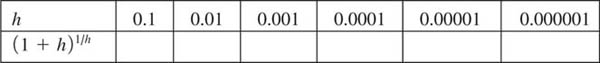
58. Use a graphing utility to graph the function f(x) = (1 + x)^1/x on the intervals [0.1, 1], [0.01, 1], and [0.001, 1]. Describe the behavior of f near x = 0.

In Problems 59 and 60, use a graphing utility as an aid in determining the x-coordinates of the points of intersection of the graphs of the functions f and g.

59. f(x) = x², g(x) = 2^x

60. f(x) = x³, g(x) = 3^x

For Discussion

61. Suppose 2^t = a and 6^t = b. Using the laws of exponents given in this Section, find the value of the given expression in terms of a and b.

(a) 12^t

(b) 3^t

(c) 6 ^−t

(d) 6^3t

(e) 2^−3t 2^7t

(f) 18^t

62. Discuss: What does the graph of look like? Do not use a graphing utility.

In Problems 63 and 64, the given fractional expression can be decomposed into partial fractions. See Section 3.6. Discuss how this can be done and carry out your ideas.

63.

64.

5.2 Logarithmic Functions

Introduction Since an exponential function y = b^x is one-to-one, we know that it has an inverse function. To find this inverse, we interchange the variables x and y to obtain x = b^y. This last formula defines y as a function of x:

y is that exponent of the base b that produces x.

By replacing the word exponent with the word logarithm, we can rephrase the preceding line as

y is that logarithm of the base b that produces x.

This last line is abbreviated by the notation y = log_b x and is called the logarithmic function.

For b > 0 there is no real number y for which b^y can either be 0 or negative. It then follows from x = b^y that x > 0. In other words, the domain of a logarithmic function y = log_b x is the set of positive real numbers (0, ∞).

For emphasis, all that is being said in the preceding sentences is:

The logarithmic expression y = log_b x and the exponential expression x = b^y are equivalent,

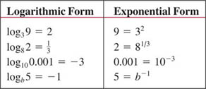
that is, they mean the same thing. As a consequence, within a specific context such as solving a problem, we can use whichever form happens to be more convenient. The following table lists several examples of equivalent logarithmic and exponential statements.

Graphs Recall from Section 2.7 that the graph of an inverse function can be obtained by reflecting the graph of the original function in the line y = x. This technique was used to obtain the red graphs from the blue graphs in FIGURE 5.2.1. As you inspect the two graphs in Figure 5.2.1(a) and in Figure 5.2.1(b), remember that the domain (−∞, ∞) and range (0, ∞) of y = b^x become, in turn, the range ( − ∞, ∞) and domain (0, ∞) of y = log_b x. Also note that the y-intercept(0, 1) for the exponential function (blue graphs) becomes the x-intercept (1, 0) for the logarithmic function (red graphs).

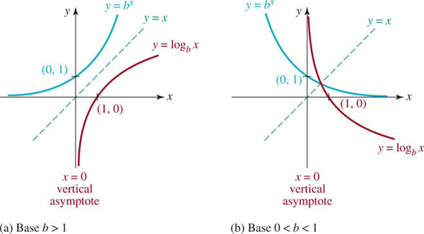
FIGURE 5.2.1 Graphs of logarithmic functions

Vertical Asymptote When the exponential function is reflected in the line y = x, the horizontal asymptote y = 0 for the graph of y = b^x becomes a vertical asymptote for the graph of y = log_b x. In Figure 5.2.1 we see that for b > 1,

whereas for 0 < b < 1,

From (7) of Section 3.5 we conclude that x = 0, which is the equation of the y-axis, is a vertical asymptote for the graph of y = log_b x.

Properties of a Logarithmic Function The following list summarizes some of the important properties of the logarithmic function f(x) = log_b x.

• The domain of f is the set of positive real numbers, that is, (0, ∞).
• The range of f is the set of real numbers, that is, (− ∞, ∞).
• The x-intercept of f is (1, 0). The graph of f has no y-intercept. (2)
• The function f is increasing for b > 1 and decreasing for 0 < b < 1.
• The y-axis, that is, x = 0, is a vertical asymptote for the graph of f.
• The function f is continuous on (0, ∞).
• The function f is one-to-one.

We would like to call attention to the third entry in the foregoing list for special emphasis:

Also,

Thus, in addition to (1, 0), the graph of any logarithmic function (1) with base b also contains the point (b, 1). The equivalence of y = log_b x and x = b^y also yields two sometimes useful identities. By substituting y = log_b x into x = b^y and then x = b^y into y = log_b x we get:

For example, from (5), 8^log₈10 = 10 and log₁₀10⁵ = 5.

EXAMPLE 1 Logarithmic Graph for b > 1

Graph f(x) = log₁₀(x + 10).

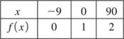
Solution This is the graph of y = log₁₀ x, which has the shape shown in Figure 5.2.1(a) shifted 10 units to the left. To reinforce the fact that the domain of a logarithmic function is the set of positive real numbers, we can obtain the domain of f(x) = log₁₀(x + 10) by the requirement that we must have x + 10 > 0 or x > −10. In interval notation, the domain of f is (−10, ∞). In the accompanying table, we have chosen convenient values of x in order to plot a few points.

Notice,

The vertical asymptote x = 0 for the graph of y = log₁₀ x becomes x = −10 for the shifted graph. This asymptote is the dashed vertical line in FIGURE 5.2.2.

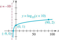
FIGURE 5.2.2 Graph of function in Example 1

Natural Logarithm Logarithms with base b = 10 are called common logarithms and logarithms with base b = e are called natural logarithms. Furthermore, it is customary to write the natural logarithm

The symbol “ln x” is usually read phonetically as “ell-en of x.” Since b = e > 1, the graph of y = lnx has the characteristic logarithmic shape shown in Figure 5.2.1(a). See FIGURE 5.2.3. For base b = e, (1) becomes

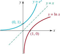
FIGURE 5.2.3 Graph of the natural logarithm

The analogues of (3) and (4) for the natural logarithm are:

The identities in (5) become

For example, from (9), e^ln13 = 13.

Common and natural logarithms can be found on all calculators.

Laws of Logarithms The laws of exponents given in Section 5.1 can be restated equivalently as the laws of logarithms. To see this, suppose we write M = b^x₁ and N = b^x₂. Then by (1), x₁ = log_bM and x₂ = log_bN.

Product: By (i) of Section 5.1, MN = b^{x₁ + x₂}. Expressed as a logarithm this is x₁ + x₂ = log_b MN. Substituting for x₁ and x₂ gives

Quotient: By (ii) of Section 5.1, M/N = b^{x₁ − x₂}. Expressed as a logarithm this is x₁ − x₂ = log_b(M/N). Substituting for x₁ and x₂ gives

Power: By (iv) of Section 5.1, M^c = b^cx₁. Expressed as a logarithm this is cx₁ = log_bM^c. Substituting for x₁ gives

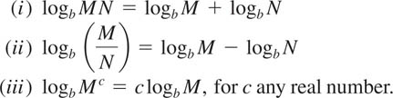
For convenience and future reference, we summarize these product, quotient, and power laws of logarithms next.

EXAMPLE 2 Laws of Logarithms

Simplify and write as a single logarithm

Solution There are several ways to approach this problem. Note, for example, that the second and third terms can be combined arithmetically as

Alternatively, we can use law (iii) followed by law (ii) to combine these terms:

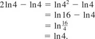
EXAMPLE 3 Rewriting Logarithmic Expressions

Use the laws of logarithms to rewrite each expression and evaluate.

(a)     (b) ln5e    (c)

Solution

(a) Since , we have from (iii) of the laws of logarithms:

(b) From (i) of the laws of logarithms and a calculator:

(c) From (ii) of the laws of logarithms:

Note that (iii) of the laws of logarithms can also be used here:

One-to-One Property The logarithmic analogue of the one-to-one property of exponential functions, (6) of Section 5.1, is:

As illustrated in Section 5.1 for the exponential function y = b^x, the one-to-one property for the logarithmic function can be used to solve certain types of equations.

EXAMPLE 4 Using the One-to-One Property

Solve ln2 + ln(4x − 1) = ln(2x + 5) for x.

Solution By (i) of the laws of logarithms, the left-hand side of the equation can be written

The original equation is then

Since two logarithms with the same base are equal, it follows immediately from the one-to-one property (10) that

Solving Equations Example 4 illustrates just one of several procedures that we can now use to solve a variety of exponential and logarithmic equations. Here is a brief list of equation-solving strategies:

• Use the one-to-one properties of b^x and log_bx.
• Rewrite an exponential expression as a logarithmic expression.
• Rewrite a logarithmic expression as an exponential expression.
• For equations a^x₁ = b^x₂, where a ≠ b, take the natural logarithm of both sides and simplify using (iii) of the laws of logarithms.

EXAMPLE 5 Rewriting an Exponential Expression

Solve e^10k = 7 for k.

Solution We use (6) to rewrite the given exponential expression as a logarithmic expression:

Therefore, with the aid of a calculator,

EXAMPLE 6 Rewriting a Logarithmic Expression

Solve log₂x = 5 for x.

Solution We use (1) to rewrite the logarithm statement in its equivalent exponential form:

EXAMPLE 7 Taking the ln of Both Sides

Solve e^2x = 3^x2⁴for x.

Solution Since the bases of the exponential expression on each side of the equality are different, one way to proceed is to take the natural logarithm (the common logarithm could also be used) of both sides. From the equality

and (iii) of the laws of logarithms, we get

Now using ln e = 1 and the distributive law, the last equation becomes

Gathering the terms involving the symbol x to one side of the equality then gives

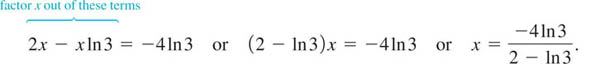
You are encouraged to verify the calculation that x ≈ −4.8752.

Change of Base Suppose we want the x-intercept of the graph of y = 2^x − 5. See FIGURE 5.2.4. By setting y = 0, we see that x is the solution of the equation 2^x − 5 = 0 or 2^x = 5. Now a perfectly valid solution is x = log₂ 5. But from a computational viewpoint (that is, expressing x as a number), the last answer is not desirable since no calculator has a logarithmic function with base 2. We can compute the answer by changing log₂ 5 to the natural logarithm by simply taking the natural log of both sides of the exponential equation 2^x = 5:

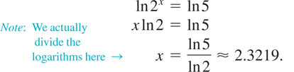
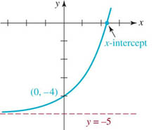
FIGURE 5.2.4 x-intercept of y = 2^x − 5

By the way, since we started with x = log₂5, the last result also proves the equality

EXAMPLE 8 Changing the Base

Find the x in the domain of f(x) = 8^x for which f(x) = 73.

Solution We must find a solution of the equation 8^x = 73. Taking the natural logarithm of both sides of the last equation and solving for x yields

With the aid of a calculator, we find . As in the discussion that precedes this example, we have actually changed bases from x = log₈73 to x = .

To convert a logarithm with any base b > 0 to the natural logarithm, we first rewrite the logarithmic expression x = log_bN as an equivalent exponential expression b^x = N. We then take the natural logarithm of both sides of the last equality and solve the resulting equation xlnb = lnN for x This yields the general formula:

NOTES FROM THE CLASSROOM

 (i) Students often struggle with the concept of a logarithm. It may help if you repeat to yourself a few dozen times, “A logarithm is an exponent.” It may also help if you begin reading a statement such as 3 = log₁₀1000 as “3 is the exponent of 10 that.…”

 (ii) For logarithmic equations of the kind in Example 4, you should get accustomed to checking your answer by substituting it back into the original equation. It is possible for a logarithmic equation to have an extraneous solution. Now work Problems 57 and 58 in Exercises 5.2.

(iii) Be very careful applying the laws of logarithms. The logarithm does not distribute over addition. In other words,

In general, there is no way that we can rewrite either

(iv) In calculus, the first step in a procedure known as logarithmic differentiation requires the student to take the natural logarithm of both sides of a complicated function such as . The idea is to use the laws of logarithms to transform powers into constant multiples, products into sums, and quotients into differences. See Problems 51–54 in Exercises 5.2.

(v) As you advance through higher courses in mathematics, science, and engineering, you may see different notations for the natural exponential function and for the natural logarithm. For example, on some calculators you may see y = exp x instead of y = e^x. In the computer algebra system Mathematica the natural exponential function is written Exp [x] and the natural logarithm is written Log[x].

5.2 Exercises
Answers to selected odd-numbered problems begin on page ANS–17.

In Problems 1–6, rewrite the given exponential expression as an equivalent logarithmic expression.

1.

2. 9⁰ = 1

3. 10⁴ = 10,000

4. 10^0.3010 = 2

5. t ^−s = v

6. (a + b)² = a² + 2ab + b²

In Problems 7–12, rewrite the given logarithmic expression as an equivalent exponential expression.

7. log₂128 = 7

8.

9.

10.

11. log_bu = v

12. log_bb² = 2

In Problems 13–18, find the exact value of the given logarithm.

13. log₁₀(0.0000001)

14. log₄64

15. log₂(2² + 2²)

16.

17. lne^e

18. ln(e⁴e⁹)

In Problems 19–22, find the exact value of the given expression.

19.

20. 25^log₅8

21. e ⁻¹ⁿ⁷

22.

In Problems 23 and 24, find a logarithmic function f(x) = log_b x such that the graph of f passes through the given point.

23. (49, 2)

24.

In Problems 25–32, find the domain of the given function f. Find the x-intercept and the vertical asymptote of the graph. Sketch the graph of f.

25. f(x) = −log₂x

26. f(x) =−log₂(x + 1)

27. f(x) = log₂(−x)

28. f(x) = log₂(3 − x)

29. f(x) = 3 − log₂(x + 3)

30. f(x) = 1 − 2log₄(x − 4)

31. f(x) = − 1 + lnx

32. f(x) = 1 + ln(x − 2)

In Problems 33 and 34, use a graph to solve the given inequality.

33. ln(x + 1) < 0

34. log₁₀(x + 3) > 1

35. Show that f(x) = ln | x | is an even function. Sketch the graph of f. Find the x-intercepts and the vertical asymptote of the graph.

36. Use the graph obtained in Problem 35 to sketch the graph of y = ln | x − 2|. Find the x-intercept and the vertical asymptote of the graph.

In Problems 37 and 38, sketch the graph of the given function f.

37. f(x) = |ln x|

38. f(x) = |ln(x + 1)|

In Problems 39–44, find the domain of the given function f.

39. f(x) = ln(2x − 3)

40. f(x) = ln(3 − x)

41. f(x) = ln(9 − x²)

42. f(x) = ln(x² − 2x)

43.

44.

In Problems 45–50, use the laws of logarithms to rewrite the given expression as one logarithm.

45. log₁₀2 + 2log₁₀5

46.

47. ln(x⁴ − 4) − ln(x² + 2)

48.

49. ln5 + ln5² + ln5³ − ln5⁶

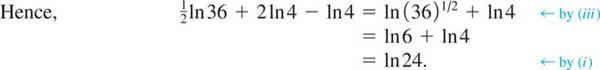
50. 5ln2 + 2ln3 − 3ln4

In Problems 51–54, use the laws of logarithms so that ln y contains no products, quotients, or powers.

51.

52.

53.

54.

In Problems 55–60, use the one-to-one property (10) to solve the given logarithmic equation.

55. log₂x − log₂10 = log₂9.3

56. ln3 + ln(2x − 1) = ln4 + ln(x + 1)

57. lnx + ln(x − 2) = ln3

58. ln(x + 3) + ln(x − 4) − lnx = ln3

59. log₂(x − 3) − log₂(2x + 1) = − log₂4

60. log₆3x − log₆(x + 1) = log₆1

In Problems 61–64, either factor or use the quadratic formula to solve the given equation.

61. (5^x)² − 2(5^x) − 1=0

62. 2^2x − 12(2^x) + 35 = 0

63. (lnx)² + lnx = 2

64. (log₁₀2x)² = log₁₀(2x)²

In Problems 65–72, use the properties of logarithms to solve the given equation.

65.

66.

67. log₂(log₃x) = 2

68. log₅ |1 − x| = 1

69. log₂(10x − x²) = 4

70. log₃(x² + 1) = 4

71. log₃81^x − log₃2^2x = 3

72.

In Problems 73 and 74, use the natural logarithm to find x in the domain of the given function for which f takes on the indicated value.

73. f(x) = 6^x; f(x) = 51

74.

In Problems 75–78, use the natural logarithm to find x.

75. 2^x+5 = 9

76. 4 · 7^2x = 9

77. 5^x = 2e^{x + 1}

78.3^{2(x −1)} = 2^{x −3}

79. In science it is sometimes useful to display data using logarithmic coordinates. Which of the following equations determines the graph shown in FIGURE 5.2.5?

 (i) y = 2x + 1

 (ii) y = e + x²

(iii) y = ex²

(iv) x²y = e

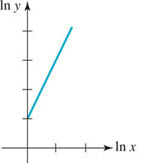
FIGURE 5.2.5 Graph for Problem 79

For Discussion

80. If a > 0 and b > 0, a ≠ b, then log_a is a constant multiple of log_b x. That is, log_a x = klog_b x. Find k.

81. Show that (log₁₀e)(log_e10) = 1. Can you generalize this result?

82. Discuss: How can the graphs of the given function be obtained from the graph of f(x) = ln x by means of a rigid transformation (a shift or a reflection)?

(a) y = ln5x

(b)

(c) y = lnx⁻¹

(d) y = ln(− x)

5.3 Exponential and Logarithmic Models

Introduction In this Section we consider some mathematical models. Roughly speaking, a mathematical model is a mathematical description of something that we will call a system. To construct a mathematical model we start with a set of reasonable assumptions about the system that we are trying to describe. These assumptions include any empirical laws that are applicable to the system. The end result could be a description as simple as a single function.

Exponential Models In the physical sciences, the exponential expression Ce^kt, where C and k are constants, frequently appears in mathematical models of systems that change with time t. As a consequence, mathematical models are often used to predict a future state of a system. For example, extremely complicated mathematical models are used to predict the weather over various regions of the country for, say, the next week.

Population Growth In one model of a growing population, it is assumed that the rate of growth of the population is proportional to the number present at time t. If P(t) denotes the population or number present at time t, then with the aid of calculus it can be shown that this assumption gives rise to

where t is time, and P₀ and k are constants. The function (1) is used to describe the growth of populations of bacteria, small animals, and, in some rare circumstances, humans. Setting t = 0 gives P(0) = P₀, and so P₀ is called the initial population. The constant k > 0 is called the growth constant or growth rate. Since e^kt, k > 0, is an increasing function on the interval [ 0, ∞) the model in (1) describes uninhibited growth.

EXAMPLE 1 Bacterial Growth

It is known that the doubling time* of E. coli bacteria, which reside in the large intestine of healthy people, is just 20 minutes. Use the exponential growth model (1) to find the number of E. coli bacteria in a culture after 6 hours.

E. coli bacteria

Solution Let us use hours as our unit of time, so that . Because the initial number of E. coli in the culture is not specified, we will simply denote the initial size of the culture as P₀. Now using (1), a function interpretation of the first sentence in this example is . This means P₀e^k/3 = 2P₀ or e^k/3 = 2. Solving this last equation for k gives the growth constant

A model for the size of the culture after t hours is then P(t) = P₀e^2.0794t. Setting t = 6 gives P(6) = P₀e^2.07946 ≈ 262,144 P₀. Put another way, if the culture consists of only one bacterium at t = 0, then (with P₀ = 1) the model predicts that there will be 262,144 cells 6 hours later.

In the early nineteenth century the English clergyman and economist Thomas R. Malthus used the growth model (1) to predict the world population. For specific values of P₀ and k, the function values P(t) were actually reasonable approximations to the world population for a period of time during the nineteenth century. Since P(t) is an increasing function, Malthus predicted that the future population growth would surpass the world’s ability to produce food. As a consequence he also predicted wars and worldwide famine. More a doomsayer than a seer, Malthus failed to foresee that the food supply would keep pace with the increased population through simultaneous advances in science and technology.

In 1840 a more realistic model for predicting human populations in small countries was advanced by the Belgian mathematician/biologist P.F. Verhulst (1804–1849). The so-called logistic function

where K, c, and r are constants, has over the years proved to be an accurate growth model for populations of protozoa, bacteria, fruit flies, water fleas, and animals confined to limited spaces. In contrast to the uninhibited growth of the Malthusian model (1), (2) exhibits bounded growth. More specifically, the population predicted by (2) will not increase beyond the number K, called the carrying capacity of the system. For r < 0, e^rt → 0 and P(t) → K as t → ∞. You are asked to examine special cases of (2) in Problems 7 and 8 in Exercises 5.3.

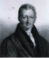
Thomas R. Malthus (1776–1834)

Radioactive Decay Element 88, better known as radium, is radioactive. This means that a radium atom spontaneously decays, or disintegrates, by emitting radiation in the form of alpha particles, beta particles, and gamma rays. When an atom disintegrates in this manner, its nucleus is transmuted into a nucleus of another element. The nucleus of the radium atom is transmuted into the nucleus of a radon atom. Radon is an odorless and colorless, but highly dangerous, radioactive gas that usually originates in the ground. Since it can penetrate a sealed concrete floor, radon frequently accumulates in basements of some new and highly insulated homes. Some medical organizations have claimed that radon is the second leading cause of lung cancer.

If it is assumed that the rate of decay of a radioactive substance is proportional to the amount remaining or present at time t, then we arrive at basically the same model as in (1). The important difference is that k < 0. If A(t) represents the amount of the decaying substance that remains at time t, then

Madame Curie (1867–1934), discoverer of radium

where A₀ is the initial amount of the substance present, that is, A(0) = A₀. The constant k < 0 in (3) is called the decay constant or decay rate.

When working problems such as this, be sure to store the value of k in the memory of your calculator.

EXAMPLE 2 Decay of Radium

Suppose there are 20 grams of radium on hand initially. After t years the amount remaining is modeled by the function A(t) = 20e^−0.000418t. Find the amount of radium remaining after 100 years. What percent of the original 20 grams has decayed after 100 years? Solution Using a calculator, we find that after 100 years there remains

Thus, only

of the initial 20 grams has decayed.

Half-Life The half-life of a radioactive substance is the time T it takes for one-half of a given amount of that element to disintegrate and change into a new element. See FIGURE 5.3.1. Half-life is a measure of the stability of an element, that is, the shorter the half-life, the more unstable the element. For example, the half-life of the highly radioactive strontium 90, Sr-90, produced in nuclear explosions, is 29 days, whereas the half-life of the uranium isotope U-238 is 4,560,000 years. The half-life of californium, Cf-244, first discovered in 1950, is only 45 minutes. Polonium, Po-213, has a half-life of 0.000001 second.

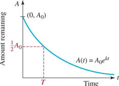
FIGURE 5.3.1 Time Tis the half-life

EXAMPLE 3 Half-Life of Radium

Use the exponential model in Example 2 to determine the half-life of radium.

Solution If A(t) = 20e^−0.000418t, then we must find the time T for which

From 20e^−0.000418T = 10 we get . By rewriting the last expression in the logarithmic form we can solve for T:

A careful reading of Example 3 reveals that the initial amount present plays no part in the actual calculation of the half-life. Since the solution of , we see that T is independent of A₀. Thus the half-life of 1 gram, 20 grams, or 10,000 grams of radium is the same. It takes about 1660 years for one-half of any given quantity of radium to transmute into radon.

Medications also have half-lives. In this case, the half-life of a drug is the time T that it takes for the body to eliminate, by metabolism or excretion, one-half of the amount of the drug taken. For example, the most popular NSAIDs (nonsteroidal antiinflammatory drugs, such as aspirin and ibuprofen) taken for the relief of continuing pain have relatively short half-lives of a few hours, and as a consequence must be taken several times a day. The NSAID naproxen has a longer half-life and is usually taken once every 12 hours.

Ibuprofen is an NSAID

Carbon Dating The approximate age of fossils of once-living matter can be determined by a method known as carbon dating. The radioactive isotope of carbon, carbon 14 or C-14, is formed presumably at a constant rate in the atmosphere by the interaction of cosmic rays on nitrogen 14. The carbon dating method, invented by the chemist Willard Libby around 1950, is based on the fact that a plant or an animal absorbs C-14 through the process of breathing and eating, and ceases to absorb C-14 when it dies. As the next example shows, the carbon dating procedure is based on the knowledge that the half-life of C-14 is about 5730 years. Carbon 14 decays back to the original nitrogen 14.

Willard Libby (1908–1980)

Libby won the 1960 Nobel prize in chemistry for his work. Libby’s method has been used to date wooden furniture found in Egyptian tombs, the Dead Sea scrolls written on papyrus and animal skin, the famous linen Shroud of Turin, and a recently discovered copy of the Gnostic Gospel of Judas written on papyrus.

The Psalms scroll

EXAMPLE 4 Carbon Dating a Fossil

A fossilized bone is found to contain of the initial amount of C-14 that the organism contained while it was alive. Determine the approximate age of the fossil.

Solution If there was an initial amount of A₀ grams of C-14 in the organism, then t years after its death there are grams remaining. When t = 5730, and so . Solving this last equation for the decay constant k gives

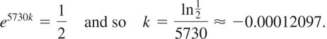
Hence a model for the amount of C-14 remaining is A(t) = A₀e^{−0.00012097t}. Using this model, we now solve for t:

The age determined in the last example is actually beyond the border of accuracy for the carbon 14 dating method. After 9 half-lives of the isotope, or about 52,000 years, about 99.7% of carbon 14 has decayed, making its measurement in a fossil nearly impossible.

Newton’s Law of Cooling/Warming Suppose an object or body is placed in a medium (air, water, etc.) that is held at constant temperature T_m, called the ambient temperature. If the initial temperature T₀ of the body or object at the moment it is placed into the medium is greater than the ambient temperature T_m, then the body will cool. On the other hand, if T₀ is less than T_m, then it will warm up. For example, in an office kept at, say, 70°F, a steaming cup of coffee will cool off, whereas a glass of ice water will warm up. The usual cooling/warming assumption is that the rate at which an object cools/warms is proportional to the difference T(t) − T_m, where T(t) represents the temperature of the object at time t. In either case, cooling or warming, this assumption leads to T(t) − T_m = (T₀ − T_m)e^kt, where k is a negative constant. Observe that since e^kt → 0 for k < 0, the last expression is consistent with one’s intuitive expectation that T(t) − T_m → 0, or equivalently T(t) → T_m, as t → ∞ (the coffee cools to room temperature; the ice water warms to room temperature). Solving for T(t) we obtain a function for the temperature of the object,

The mathematical model in (4), named after its discoverer, is called Newton’s law of cooling/warming.

EXAMPLE 5 Cooling of a Cake

A cake is removed from an oven where the temperature was 350°F into a kitchen where the temperature is 75°F. One minute later the temperature of the cake is measured to be 300°F.

(a) What is the temperature of the cake after 6 minutes?

(b) At what time is the temperature of the cake 80°F?

(c) Graph T(t).

Cake will cool to room temperature

Solution (a) When the cake is removed from the oven its temperature is also 350°F, that is, T₀ = 350. The ambient temperature is the temperature of the kitchen, T_m = 75. Thus (4) becomes T(t) = 75 + 275e^kt. The measurement that T(1) = 300 is the condition that determines k. From

From the model T(t) = 75 + 275e^−0.2007twe then find

(b) To determine when the temperature of the cake will be 80°F, we solve the equation T(t) = 80 for t. Rewriting T(t) = 75 + 275e^−0.2007t = 80 as

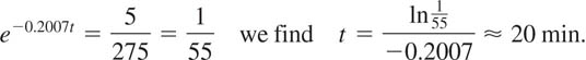
(c) With the aid of a graphing utility we obtain the graph of T(t) shown in blue in FIGURE 5.3.2. Since T(t) = 75 + 275e^−0.2007t → 75 as t → ∞, T = 75, shown in red in Figure 5.3.2, is a horizontal asymptote for the graph of T(t) = 75 + 275e ^−0.2007t.

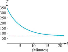
FIGURE 5.3.2 Graph of T(t) in Example 5

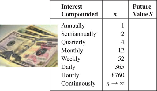
Compound Interest Investments such as savings accounts pay an annual rate of interest that can be compounded annually, quarterly, monthly, weekly, daily, and so on. In general, if a principal of P dollars is invested at an annual rate r of interest that is compounded n times a year, then the amount S accrued at the end of t years is given by

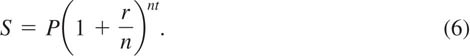
S is called the future value of the principal P. If the number n is increased without bound, then interest is said to be compounded continuously. To find the future value of P in this case, we let m = n/r. Then n = mr and

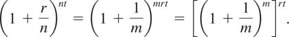
Since n → ∞ implies that m → ∞, we see from (3) of Section 5.1 that (1 + 1 /m)^m → e. The right-hand side of (6) becomes

Thus, if an annual rate r of interest is compounded continuously, the future value S of a principal P in t years is

EXAMPLE 6 Comparing Future Values

Suppose that $1000 is deposited in a savings account whose annual rate of interest is 3%. Compare the future value of this principal in 10 years (a) if interest is compounded monthly and (b) if interest is compounded continuously.

Solution

(a) Since there are 12 months in a year, we identify n = 12. Furthermore, with P = 1000, r = 0.03, and t = 10, (6) becomes

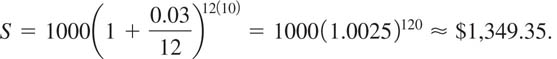
(b) From (7),

Thus over 10 years we have gained $0.51 by compounding continuously rather than monthly.

Logarithmic Models Probably the most famous application of the base 10 logarithm, or common logarithm, is the Richter scale. In 1935 the American seismologist Charles F. Richter devised a logarithmic scale for comparing the energies of different earthquakes. The magnitude M of an earthquake is defined by

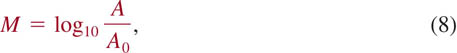
where A is the amplitude of the largest seismic wave of the earthquake and A₀ is a reference amplitude that corresponds to the magnitude M = 0. The number M is calculated to one decimal place. Earthquakes of magnitude 6 or greater are considered potentially destructive.

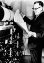
Charles F. Richter (1900–1985)

EXAMPLE 7 Comparing Intensities

The earthquake on December 26, 2004, off of the west coast of Northern Sumatra, which spawned a tsunami causing over 200,000 deaths, was initially classified a 9.3 on the Richter scale. On March 28, 2005, an aftershock in the same area was classified as an 8.7 on the Richter scale. How many times more intense was the 2004 earthquake?

Solution From (8) we have

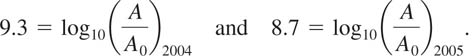
This means, in turn, that

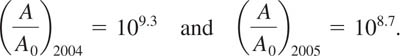
Now, since 9.3 = 8.7 + 0.6, it follows from the laws of exponents that

Thus the original earthquake in 2004 was approximately 4 times as intense as the aftershock in 2005.

You can see from Example 7 that if, say, one earthquake is a 6.0 and another is a 4.0 on the Richter scale, then the 6.0 earthquake is 10² = 100 times more intense than the 4.0 earthquake.

pH of a Solution In chemistry, the hydrogen potential, or pH, of a solution is defined as

where the symbol [H⁺] denotes the concentration of hydrogen ions in solution measured in moles per liter. The pH scale was invented in 1909 by the Danish biochemist Søren Sørensen. Solutions are classified according to their pH value as acidic, base, or neutral. A solution with a pH in the range 0 < pH < 7 is said to be acid; when pH > 7, the solution is base (or alkaline). In the case when pH = 7, the solution is neutral. Water, if uncontaminated by other solutions or by acid rain, is an example of a neutral solution, whereas undiluted lemon juice is highly acid and has a pH in the range pH ≤ 3. A solution with pH = 6 is ten times more acidic than a neutral solution. See Problems 47–50 in Exercises 5.3.

Søren Sørensen (1868–1939)

As the next example illustrates, pH values are usually calculated to one decimal place.

EXAMPLE 8 pH of Human Blood

The concentration of hydrogen ions in the blood of a healthy person is found to be [H⁺] = 3.98 × 10⁻⁸ moles/liter. Find the pH of blood.

Solution From (9) and the laws of logarithms,

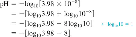
With the help of the base-10 log key on a calculator, we find that

Human blood in usually a base solution. The pH values of blood usually fall within the rather narrow range 7.2 < pH < 7.6. A person with a blood pH outside these limits can suffer illness and even death.

5.3 Exercises
Answers to selected odd-numbered problems begin on page ANS–17.

Population Growth

1. After 2 hours the number of bacteria in a culture is observed to have doubled.

(a) Find an exponential model (1) for the number of bacteria in the culture at time t.

(b) Find the number of bacteria present in the culture after 5 hours.

(c) Find the time that it takes the culture to grow to 20 times its initial size.

2. A model for the number of bacteria in a culture after t hours is given by (1).

(a) Find the growth constant k if it is known that after 1 hour the colony has expanded to 1.5 times its initial population.

(b) Find the time that it takes for the culture to quadruple in size.

3. A model for the population in a small community is given by P(t) = 1500e^kt. If the initial population increases by 25% in 10 years, what will the population be in 20 years?

4. A model for the population in a small community after t years is given by (1).

(a) If the initial population has doubled in 5 years, how long will it take to triple? To quadruple?

(b) If the population of the community in part (a) is 10,000 after 3 years, what was the initial population?

5. A model for the number of bacteria in a culture after t hours is given by P(t) = P₀e^kt. After 3 hours it is observed that 400 bacteria are present. After 10 hours 2000 bacteria are present. What was the initial number of bacteria?

6. In genetic research a small colony of drosophila (small two-winged fruit flies) is grown in a laboratory environment. After 2 days it is observed that the population of flies in the colony has increased to 200. After 5 days the colony has 400 flies.

(a) Find a model P(t) = P₀e^kt for the population of the fruit-fly colony after t days.

(b) What will be the population of the colony in 10 days?

(c) When will the population of the colony be 5000 fruit flies?

7. A student sick with a flu virus returns to an isolated college campus of 2000 students. The number of students infected with the flu t days after the student’s return is predicted by the logistic function

(a) According to this model, how many students will be infected with the flu after 5 days?

(b) How long will it take for one-half of the student population to become infected?

(c) How many students does the model predict will become infected after a very long period of time?

(d) Sketch a graph of P(t).

8. In 1920, Pearl and Reed proposed a logistic model for the population of the United States based on the years 1790, 1850, and 1910. The logistic function they proposed was

where P is measured in thousands and t represents the number of years past 1780.

(a) The model agrees quite well with the census figures between 1790 and 1910. Determine the population figures for 1790, 1850, and 1910.

(b) What does this model predict for the population of the United States after a very long time? How does this prediction compare with the 2000 census population of 281 million?

Radioactive Decay and Half-Life

9. Initially 200 milligrams of a radioactive substance was present. After 6 hours the mass had decreased by 3%. Construct an exponential model A(t) = A₀e^kt for the amount remaining of the decaying substance after t hours. Find the amount remaining after 24 hours.

10. Determine the half-life of the substance in Problem 9.

11. Do this problem without using the exponential model (3). Initially there are 400 grams of a radioactive substance on hand. If the half-life of the substance is 8 hours, give an educated guess of how much remains (approximately) after 17 hours. After 23 hours. After 33 hours.

12. Construct an exponential model A(t) = A₀e^kt for the amount remaining of the decaying substance in Problem 11. Compare the predicted values A(17), A(23), and A(33) with your guesses.

13. Iodine 131, used in nuclear medicine procedures, is radioactive and has a half-life of 8 days. Find the decay constant k for iodine 131. If the amount remaining of an initial sample after t days is given by the exponential model A(t) = A₀e^kt, how long will it take for 95% of the sample to decay?

14. The amount remaining of a radioactive substance after t hours is given by A(t) = 100e^kt. After 12 hours, the initial amount has decreased by 7%. How much remains after 48 hours? What is the half-life of the substance?

15. The half-life of polonium 210, Po-210, is 140 days. If A(t) = A₀e^kt represents the amount of Po-210 remaining after t days, what is the amount remaining after 80 days? After 300 days?

16. Strontium 90 is a dangerous radioactive substance found in acid rain. As such it can make its way into the food chain by polluting the grass in a pasture on which milk cows graze. The half-life of strontium 90 is 29 years.

(a) Find an exponential model (3) for the amount remaining after t years.

(b) Suppose a pasture is found to contain Str-90 that is 3 times a safe level A₀. How long will it be before the pasture can be used again for grazing cows?

Carbon Dating

17. Charcoal drawings were discovered on walls and ceilings in a cave in Lascaux, France. Determine the approximate age of the drawings if it was found that 86% of C-14 in a piece of charcoal found in the cave had decayed through radioactivity

Charcoal drawing in Problem 17

18. Analysis of an animal bone fossil at an archeological site reveals that the bone has lost between 90% and 95% of C-14. Give an interval for the possible ages of the bone.

19. The shroud of Turin shows the negative image of the body of a man who appears to have been crucified. It is believed by many to be the burial shroud of Jesus of Nazareth. In 1988 the Vatican granted permission to have the shroud carbon dated. Several independent scientific laboratories analyzed the cloth and the consensus opinion was that the shroud is approximately 660 years old, an age consistent with its historical appearance. This age has been disputed by many scholars. Using this age, determine what percentage of the original amount of C-14 remained in the cloth as of 1988.

Shroud image in Problem 19

20. In 1991 hikers found a preserved body of a man partially frozen in a glacier in the Austrian Alps. Through carbon dating techniques it was found that the body of Ötzi—as the iceman came to be called—contained 53% as much C-14 as found in a living person. What is the approximate date of his death?

The iceman in Problem 20

Newton’s Law of Cooling/Warming

21. Suppose a pizza is removed from an oven at 400°F into a kitchen whose temperature is a constant 80°F. Three minutes later the temperature of the pizza is found to be 275°F.

(a) What is the temperature T(t) of the pizza after 5 minutes?

(b) Determine the time when the temperature of the pizza is 150°F.

(c) After a very long period of time, what is the approximate temperature of the pizza?

22. A glass of cold water is removed from a refrigerator whose interior temperature is 39°F into a room maintained at 72°F. One minute later the temperature of the water is 43°F. What is the temperature of the water after 10 minutes? After 25 minutes?

23. A thermometer is brought from the outside, where the air temperature is − 20°F, into a room where the air temperature is a constant 70°F. After one minute inside the room the thermometer reads 0°F. How long will it take for the thermometer to read 60°F?

24. A thermometer is taken from inside a house to the outside, where the air temperature is 5°F. After one minute outside the thermometer reads 59°F, and after 5 minutes it reads 32°F. What is the temperature inside the house?

Thermometer in Problem 24

25. A dead body was found within a closed room of a house where the temperature was a constant 70°F. At the time of discovery, the core temperature of the body was determined to be 85°F. One hour later a second measurement showed that the core temperature of the body was 80°F. Assume that the time of death corresponds to t = 0 and that the core temperature at that time was 98.6°F. Determine how many hours elapsed before the body was found.

26. Repeat Problem 25 if evidence indicated that the dead person was running a fever of 102°F at the time of death.

Compound Interest

27. Suppose that 1¢ is deposited in a savings account paying 1% annual interest compounded continuously. How much money will have accrued in the account after 2000 years? What is the future value of 1¢ in 2000 years if the account pays 2% annual interest compounded continuously?

28. Suppose that $100,000 is invested at an annual rate of interest of 5%. Use (6) and (7) to compare the future values of that amount in 1 year by completing the following table.

29. Suppose that $5000 is deposited in a savings account paying 6% annual interest compounded continuously. How much interest will be earned in 8 years?

30. If (7) is solved for P, that is, P = Se^−rt, we obtain the amount that should be invested now at an annual rate r of interest in order to be worth S dollars after t years. We say that P is the present value of the amount S. What is the present value of $100,000 at an annual rate of 3% compounded continuously for 30 years?

Miscellaneous Exponential Models

31. Effective Half-life Radioactive substances are removed from living organisms by two processes: natural physical decay and biological metabolism. Each process contributes to an effective half-life E that is defined by

where P is the physical half-life of the radioactive substance and B is the biological half-life.

(a) Radioactive iodine, I-131, is used to treat hyperthyroidism (overactive thyroid). It is known that for human thyroids, P = 8 days and B = 24 days. Find the effective half-life of I-131.

(b) Suppose the amount of I-131 in the human thyroid after t days is modeled by A(t) = A₀e^kt, k < 0. Use the effective half-life found in part (a) to determine the percentage of radioactive iodine remaining in the human thyroid gland two weeks after its ingestion.

32. Newton’s Law of Cooling Revisited The rate at which a body cools also depends on its exposed surface area S. If S is a constant, then a modification of (4) is

Suppose two cups A and B are filled with coffee at the same time. Initially the temperature of the coffee is 150°F. The exposed surface area of the coffee in cup B is twice the surface area of the coffee in cup A. After 30 min, the temperature of the coffee in cup A is 100°F. If T_m = 70°F, what is the temperature of the coffee in cup B after 30 min?

33. Series Circuit In a simple series circuit consisting of a constant voltage E, an inductance of L henries, and a resistance of R ohms, it can be shown that the current I(t) is given by

Solve for t in terms of the other symbols.

34. Drug Concentration Under some conditions the concentration of a drug at time t after ingestion is given by

Here a and b are positive constants and C₀ is the concentration of the drug at t = 0. Determine the steady-state concentration of a drug, that is, the limiting value of C(t) as t → ∞. Determine the time t at which C(t) is one-half the steady-state concentration.

Richter Scale

35. Two of the most devastating earthquakes in the San Francisco Bay area occurred in 1906 along the San Andreas fault and in 1989 in the Santa Cruz Mountains near Loma Prieta peak. The 1906 and 1989 earthquakes measured 8.5 and 7.1 on the Richter scale, respectively. How much greater was the intensity of the 1906 earthquake compared to the 1989 earthquake?

Marina district in San Francisco, 1989

36. How much greater was the intensity of the 2004 Northern Sumatra earthquake (Example 7) compared to the 1964 Alaskan earthquake of magnitude 8.9?

37. If an earthquake has a magnitude 4.2 on the Richter scale, what is the magnitude on the Richter scale of an earthquake that has an intensity 20 times greater? [Hint: First solve the equation 10^x 5 20.]

38. Show that the Richter scale defined in (8) of this Section can be written

pH of a Solution

In Problems 39−42, determine the pH of a solution with the given hydrogen-ion concentration [H⁺].

39. 10⁻⁶

40. 4 × 10⁻⁷

41. 2.8 × 10⁻⁸

42. 5.1 × 10⁻⁵

In Problems 43–46, determine the hydrogen-ion concentration [H⁺] of a solution with the given pH.

43. 3.3

44. 7.3

45. 6.6

46. 8.1

In Problems 47–50, determine how many more times acidic the first substance is compared to the second substance.

47. lemon juice: pH = 2.3,    vinegar: pH = 3.3

48. battery acid: pH = 1,        lye: pH = 13

49. acid rain: pH = 3.8,         clean rain: pH = 5.6

50. NaOH: [H⁺] = 10⁻¹⁴,     HCl: [H⁺] = 1

Miscellaneous Logarithmic Models

51. Richter Scale and Energy Charles Richter, working with Beno Gutenberg, developed the model

that relates the Richter magnitude M of an earthquake and its seismic energy E (measured in ergs). Calculate the seismic energy E of the 2004 Northern Sumatra earthquake where M = 9.3.

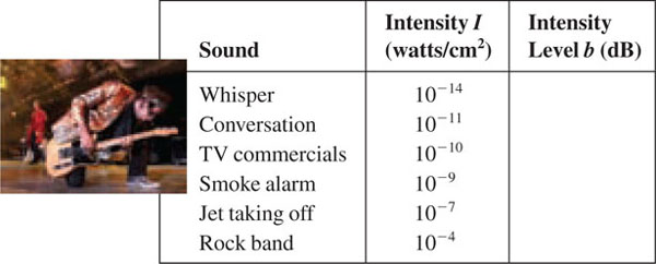
52. Intensity Level The intensity level b of a sound measured in decibels (dB) is defined by

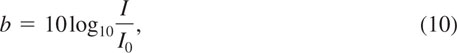
where I is the intensity of the sound measured in watts/cm² and I₀ = 10⁻¹⁶ watts/cm² is the intensity of the faintest sound that can be heard (0 dB). Use (10) and complete the following table.

53. The threshold of pain is generally taken to be around 140 dB. Find the intensity of sound I corresponding to 140 dB.

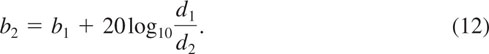
54. The intensity of sound I is inversely proportional to the square of the distance d from its source, that is,

where k is the constant of proportionality. Suppose d₁ and d₂ are distances from a source of sound, and that the corresponding intensity levels of the sounds are b₁ and b₂. Use (11) in (10) to show that b₁ and b₂ are related by

55. When a plane P₁, flying at an altitude of 1500 ft, passed over a point on the ground its intensity level b₁ was measured as 70 dB. Use (12) to find the intensity level b₂ of a second plane P₂, flying at an altitude of 2600 ft, when it passed over the same point.

56. At a distance of 4 ft, the intensity level of an animated conversation is 50 dB. Use (12) to find the intensity level 14 ft from the conversation.

57. Pupil of the Eye An empirical model devised by DeGroot and Gebhard relates the diameter d of the pupil of the eye (measured in millimeters, mm) to the luminance B of light source (measured in millilambert’s, mL):

See FIGURE 5.3.3.

FIGURE 5.3.3 Pupil diameter in Problem 57

(a) The average luminance of clear sky is approximately B = 255 mL. Find the corresponding pupil diameter.

(b) The luminance of the sun varies from approximately B = 190,000 mL at sunrise to B = 51,000,000 mL at noon. Find the corresponding pupil diameters.

(c) Find the luminance B corresponding to a pupil diameter of 7 mm.

5.4 The Hyperbolic Functions

Logarithms were invented in the late sixteenth century by the Scottish lord—and nonmathematician—John Napier (1550–1617). It was he who coined the word “logarithm” from the two Greek words logos, meaning ratio, and arithmos, meaning number or power. But it took almost two centuries and the genius of the Swiss mathematician Leonhard Euler (1707–1783) before the mathematical community became fully aware of the irrational number e and its importance. It is his work that we emulate below in showing why the number e is the natural choice of base for the exponential and logarithmic functions.

Leonard Euler

Difference Quotient Revisited We return to the difference quotient concept first introduced in Section 2.9. Recall that we compute

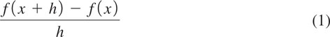
in three steps. For the exponential function f(x) = b^x, we have

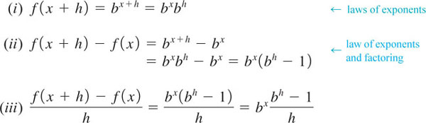
In the fourth step, the calculus step, we let h → 0 but, unlike all the problems given in Exercises 2.9, there is no apparent way of canceling the h in (iii). Nonetheless, the derivative of f(x) = b^x is

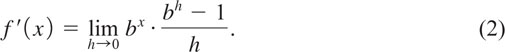
Since b^x does not depend on the variable h, we can rewrite (2) as

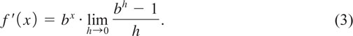
Now here are the amazing results. The limit in (3),

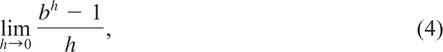
can be shown to exist for every positive base b. However, as one might expect, we will get a different answer for each base b. So let’s denote the expression in (4) by the symbol m(b). The derivative of f(x) = b^x is then

You are asked to approximate the value of m(b) in the four cases b = 1.5, 2, 3, and 5 in Problems 21–24 of Exercises 5.4. For example, it can be shown that m(10) ≈ 2.302585…, and as a consequence the derivative of f(x) = 10^x is

We can get a better understanding of what m(b) is by evaluating (5) at x = 0. Since b⁰ = 1, we have f ´(0) = m(b). In other words, m(b) is the slope of the tangent line to the graph of f(x) = b^x at x = 0, that is, at the y-intercept (0, 1). See FIGURE 5.4.1. Given that we have to calculate a different m(b) for each base b, and that m(b) is likely to be an “ugly” number as in (6), over time the following question arose naturally:

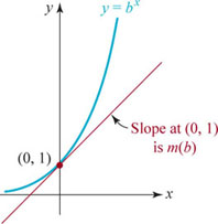
FIGURE 5.4.1 Find a base b so that the slope m1b2 of tangent line at 10, 12 is 1

The Answer To answer the question posed in (7), we must return to the definitions of e given in Section 5.1. Specifically, (4) of Section 5.1,

provides the means for answering the question posed in (7). If you have studied Sections 1.5, 2.9, and 4.11 you should have an intuitive understanding that the equality in (8) means that as h gets closer and closer to 0 then (1 + h)^1/h can be made arbitrarily close to the number e. Thus for values of h near 0, we have the approximation (1 + h)^1/h ≈ e, and so it follows that 1 + h ≈ e^h. By rewriting the last expression in the form

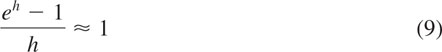
we can conclude that

Since the right-hand side of (10) is m(e), we have the answer to the question in (7):

In addition, from (3) we have discovered a wonderfully simple result: The derivative of f(x) = e^xis

The result in (12) is the same as

Moreover, the only other nonzero function f in calculus whose derivative is equal to itself is f(x) = ce^x, where c ≠ 0 is a constant.

What’s Next? Since y = log_b x and y = b^x are inverse functions, one would expect that since the simplest derivative of y = b^x is obtained when b = −e that the simplest derivative of y = log_bx also occurs for that base. That is indeed the case. You are encouraged to reexamine (3) of Section 5.1 and then work Problems 1-4 in Exercises 5.4.

Hyperbolic Functions We have already seen in Section 5.3 the usefulness of the exponential function e^x in various mathematical models. As a further application, consider a long rope or a flexible wire, such as a telephone wire hanging only under its own weight between two fixed supports. It can be shown that under certain conditions the hanging wire assumes the shape of the graph of the function

The symbol c stands for a positive constant that depends on the physical characteristics of the wire. Functions such as (13), consisting of certain combinations of e^x and e^{− x}, appear in so many applications that mathematicians have given them names. In particular, when c = 1 in (13), the resulting function is called the hyperbolic cosine.

Analogous to the trigonometric functions tanx, cotx, secx, and cscx that are defined in terms of sinx and cosx, there are four additional hyperbolic functions tanh x, coth x, sech x, and csch x that are defined in terms of sinh x and cosh x. For example, the hyperbolic tangent and hyperbolic secant functions are defined as

See Problems 21 and 22 in Exercises 5.4.

Graphs The graph of the hyperbolic cosine, shown in FIGURE 5.4.2, is called a catenary. The word catenary derives from the Latin word for a chain, catena. The shape of the famous 630-foot tall Gateway arch in St. Louis, Missouri, is an inverted catenary. Compare the shape in Figure 5.4.2 with that in the accompanying photo. The graph of y = sinh x is given in FIGURE 5.4.3.

Gateway arch in St. Louis, MO

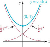
FIGURE 5.4.2 Graph of y = cosh x is a catenary

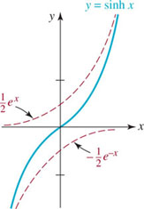
FIGURE 5.4.3 Graph of y = sinh x

Identities Although the hyperbolic functions are not periodic, they possess identities that are similar to trigonometric identities. Analogous to the basic Pythagorean identity of trigonometry sin² x + cos²x = 1, for the hyperbolic sine and cosine we have

See Problems 9–14 in Exercises 5.4.

5.4 Exercises
Answers to selected odd-numbered problems begin on page ANS–17.

1. Use the laws of logarithms to show that for f(x) = log_b x,

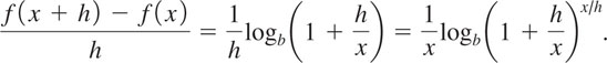
2. From Problem 1, the derivative of f(x) = log_b x is

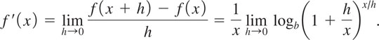
Let us assume that the limiting process can be taken inside the logarithm:

Rewrite the foregoing result using the substitution n = x/h. Notice that since x is held fixed, as h → 0 we must have n → ∞. Give the precise value off′(x).

In Problems 3 and 4, use the result of Problem 2 to find f′(x) for the given function.

3. f(x) = log₁₀ x

4. f(x) = ln x

In Problems 5 and 6, use the result of Problems 1 and 2 to find f′(x) for the given function. Before using the difference quotient, use the laws of logarithms to rewrite the function.

5.

6. f(x) = log₁₀6x

In Problems 7 and 8, compute for the given function.

7. f(x) = e^5x

8. f(x) = e ^−x+4

In Problems 9–14, use the definitions of sinh x and cosh x in (14) and (15) to verify the given identity.

9. cosh²x − sinh²x = 1

10. 1 − tanh²x = sech²x.

11. cosh(− x) = cosh x

12. sinh(−x) = −sinh x

13. sinh 2x = 2sinh x cosh x

14. cosh 2x = cosh²x + sinh²x

15. If , use the identity given in Problem 9 to find the value of sinh x.

16. If , use the identity given in Problem 10 to find the value of cosh x.

17. As can be seen in Figure 5.4.3, the hyperbolic sine function y = sinh x is one-to-one. Use the definition of the hyperbolic sine in (14) in the form e^x −2y − e ^−x = 0 to show that the inverse hyperbolic sine sinh⁻¹x can be expressed in terms of the natural logarithm:

[Hint: Interchange x and y in e^x −2y − e ^x = 0 and solve for y.]

18. (a) Use the graph of y = sinh x in Figure 5.4.3 to sketch the graph of the inverse hyperbolic sine y = sinh⁻¹x defined in Problem 17.

(b) Give the domain and range of y = sinh⁻¹x.

19. The function y = cosh x is one-to-one on the restricted domain [0, ∞). Proceed as in Problem 17 to show that the inverse hyperbolic cosine cosh⁻¹x can be expressed in terms of the natural logarithm:

20. (a) Use the graph of y = cosh x in Figure 5.4.2 to sketch the graph of the inverse hyperbolic cosine y = cosh⁻¹x defined in Problem 19.

(b) Give the domain and range of y = cosh⁻¹x.

21. The definition of the hyperbolic tangent is

Sketch the graph of y = tanh x.

22. The definition of the hyperbolic secant is

Sketch the graph of y = sech x.

23. The function y = tanh x is one-to-one. Use the graph obtained in Problem 21 to sketch the graph of the inverse hyperbolic tangent y = tanh⁻¹x. Give the domain and range of y = tanh⁻¹x.

24. The function y = sech x is one-to-one on the restricted domain [0, ∞). Use the graph obtained in Problem 22 to sketch the graph of the inverse hyperbolic secant y = sech⁻¹x. Give the domain and range of y = sech⁻¹x.

Calculator Problems

25. Use a calculator to investigate for the function in Problem 7. Determine f′(x).

26. Use a calculator to investigate for the function in Problem 8. Determine f ’(x).

In Problems 27–30, use a calculator to estimate the value for b = 1.5, b = 2, b = 3, and b = 5 by filling out the given table.

27.

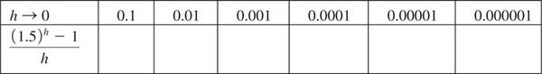
28.

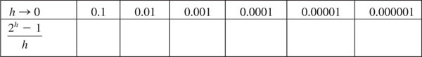
29.

30.

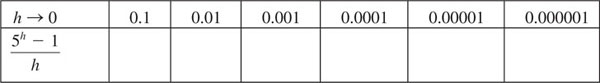
31. Fill out a table of the kind in Problems 27–30, but this time use

32. A Curiosity The logarithm developed by John Napier (see page 316) was actually

Use (11) of Section 5.2 to express this logarithm in terms of the natural logarithm.

CHAPTER 5 Review Exercises
Answers to selected odd-numbered problems begin on page ANS–17.

In Problems 1–22, fill in the blanks.

1. The graph of y = 6 − e^−x has the y-intercept______and horizontal asymptote y =________.

2. The x-intercept of the graph of y = −10 + 10^5xis______.

3. The graph of y = ln (x + 4) has the x-intercept______and vertical asymptote x =________.

4. The y-intercept of the graph of y = log₈(x + 2) is______.

5. log₅2 − log₅10 =______

6.

7. e^3ln10 =______

8. 10^{log₁₀4.89} =______

9. log₄ (4 · 4 ²· 4 ³) =______

10.

11. If log₃N = − 2, then N =______.

12.

13. If lne³ = y, then y =______.

14. If ln3 + ln(x − 1) = ln2 + lnx, then x =______.

15. If − 1 + ln(x − 3) = 0,then x =______.

16. If ln (lnx) = 1, then x =______.

17. If 100 − 20e ^−015t = 35, then to four rounded decimals t =______.

18. If 3^x = 5,then 3^−2x =______.

19. f(x) = 4^3x = (___)^x

20. f(x) = (e²)^x/6 = (___)^x

21. If the graph of y = e^x−2 + C passes through (2, 9), then C =______.

22. By rigid transformations, the point (0, 1) on the graph of y = e^x is moved to the point______on the graph of y = 4 + e^x−3.

In Problems 23–36, answer true or false.

23. y = ln x and y = e^x are inverse functions.______

24. The point (b, 1) is on the graph of f(x) = log_b x.______

25. y = 10^−x and y = (0.1)^x are the same function.______

26.

27. 4^x/2 = 2^x______

28.

29. 2^x + 2 ^−x = (2 + 2⁻¹)^x______

30. 2^{3 + 3x} = 8^{1 + x}______

31.

32.

33. ln(ln e) = 1______

34.

35. ln(e + e) = 1 + ln2______

36. log₆(36)⁻¹ = −2 ______

In Problems 37 and 38, rewrite the given exponential expression as an equivalent logarithmic expression.

37. 5⁻¹ = 0.2

38.

In Problems 39 and 40, rewrite the given logarithmic expression as an equivalent exponential expression.

39. log₉27 = 1.5

40. log₆(36)²² = −4

In Problems 41–48, solve for x.

41. 2^{1 −x} = 8

42. 3^2x = 81

43. e^{1 −2x} = e²

44.

45. 2^1−x = 7

46. 3^x = 7^{x −1}

47. e^x+2 = 6

48. 3e^x = 4e ^−3x

In Problems 49 and 50, graph the given functions on the same coordinate axes.

49. y = 4^x, y = log₄ x

50.

51. Match the letter of the graph in FIGURE 5.R.1 with the appropriate function.

 (i)  f(x) = b^x, b > 2

(ii) f(x) =b^x, 1 < b < 2

(iii)

(iv)

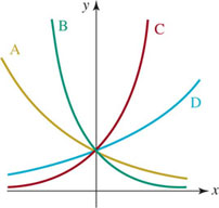
FIGURE 5.R.1 Graphs for Problem 51

52. In FIGURE 5.R.2, fill in the blanks for the coordinates of the points on each graph.

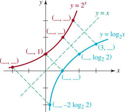
FIGURE 5.R.2 Graphs for Problem 52

In Problems 53 and 54, find the slope of the line L given in each figure.

53.

FIGURE 5.R.3 Graph for Problem 53

54.

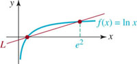
FIGURE 5.R.4 Graph for Problem 54

In Problems 55–60, match each of the following functions with one of the given graphs.

 (i) y = ln(x − 2)

(ii) y = 2 − ln x

(iii) y = 2 + ln(x + 2)

(iv) y = −2 − ln(x + 2)

(v) y = −ln(2x)

(vi) y = 2 + ln(−x + 2)

55.

FIGURE 5.R.5 Graph for Problem 55

56.

FIGURE 5.R.6 Graph for Problem 56

57.

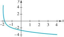
FIGURE 5.R.7 Graph for Problem 57

58.

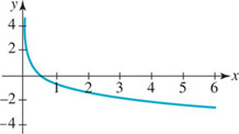
FIGURE 5.R.8 Graph for Problem 58

59.

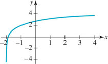
FIGURE 5.R.9 Graph for Problem 59

60.

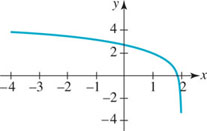
FIGURE 5.R.10 Graph for Problem 60

In Problems 61 and 62, in words describe the graph of the function f in terms of a transformation of the graph of y = ln x.

61.

62. f(x) = ln x

63. Find a function f(x) = Ae^kx if (0, 5) and (6, 1) are points on the graph of f.

64. Find a function f(x) = A10^kx if f (3) = 8 and .

65. Find a function f(x) = a + b^x,0 < b < 1,if f (1) = 5.5 and the graph of f has a horizontal asymptote y = 5.

66. Find a function f(x) = a + log₃ (x − c) if f (11) = 10 and the graph of f has a vertical asymptote x = 2.

67. If the initial number of bacteria present in a culture doubles after 9 hours, how long will it take for the number of bacteria in the culture to double again?

68. A commercial fishing lake is stocked with 10,000 fingerlings. Find a model P(t) = P₀e^kt for the fish population of the lake at time t if the owner of the lake estimates that there will be 5000 fish left after six months. After how many months does the model predict that there will be 1000 fish left?

69. Tritium, an isotope of hydrogen, has a half-life of 12.5 years. How much of an initial quantity of this element remains after 50 years?

70. It is found that 97% of C-14 has been lost in a human skeleton found at an archeological site. What is the approximate age of the skeleton?

71. A person facing retirement invests $650,000 in a savings account. She wants the account to be worth $1,000,000 in 10 years. What annual rate r of interest compounded continuously will achieve this dream?

72. According to the Beer-Lambert-Bouguer law, the intensity I (measured in lumens) of a vertical beam of light passing through a transparent substance decreases according to the exponential function I(x) = I₀e^kx, k < 0, where I₀ is the intensity of the incident beam and x is the depth measured in meters. Suppose the intensity of light 1 meter below the surface of water is 30% of I₀. What is the intensity 3 meters below the surface? At what depth is the intensity 50% of that at the surface?

73. The Gompertz function , where a, b, and c are positive constants, is named after the self-educated English mathematician Benjamin Gompertz (1779–1865) and was used initially in the study of population demographics. Today Gompertz’s function is used as a mathematical model in diverse areas such as economics, statistics, and oncological studies of the growth of tumors. Solve for t in terms of the other symbols.

74. The graph of a Gompertz function is naturally called a Gompertz curve. Sketch the Gompertz curve in the following cases. In each case, superimpose the three graphs on the same rectangular coordinate system.

(a)

(b)

(c)

[Hint: The graph has two horizontal asymptotes.]

75. An annuity is a savings plan where the same amount of money P is deposited into an account at n equally spaced periods (say, years) of time. If the annual rate r of interest is compounded continuously, then the amount S accrued in the account immediately after the nth deposit is

What is the value of such an annuity in 15 years if P = $3000 and the annual rate of interest is 2%.

---

* In biology the doubling time is sometimes referred to as the generation time.