Ethernet systems operated as half-duplex systems for many years, and a number of simulations and analyses of those systems were published. This activity resulted in a number of myths and misconceptions about the performance of older Ethernet systems, which are discussed next. Keep in mind that we are discussing the old half-duplex model of Ethernet operation, which is rarely used anymore.

When calculating the performance of a half-duplex Ethernet channel, researchers often used simulations and analytic models based on a deliberately overloaded system. This was done to see what the limits of the channel were, and how well the channel could hold up to extreme loads.

Over time, the simulations and analytic models used in these studies became increasingly sophisticated in their ability to model actual half-duplex Ethernet channel behavior. Early simulations frequently made a variety of simplifying assumptions to make the analysis easier, and ended up analyzing systems whose behavior had nothing much to do with the way a real half-duplex Ethernet functioned. This produced some odd results, and led some people to deduce that Ethernets would saturate at low utilization levels.

Due to the incorrect results coming from simplified models, there arose some persistent myths about half-duplex Ethernet performance, chief of which was that the Ethernet channel saturated at 37% utilization. We’ll begin with a look at where this figure comes from, and why it had nothing to do with real-world Ethernets.

The 37% figure was first reported by Bob Metcalfe and David Boggs in their 1976 paper that described the development and operation of the very first Ethernet.^[67] This was known as the “experimental Ethernet,” which operated at about 3 Mb/s. The experimental Ethernet frame had 8-bit address fields, a 1-bit preamble, and a 16-bit CRC field.

In this paper, Metcalfe and Boggs presented a “simple model” of performance. Their model used the smallest frame size and assumed a constantly transmitting set of 256 stations, which was the maximum supported on experimental Ethernet. Using this simple model, the system reached saturation at about 36.8% channel utilization. The authors warned that this was a simplified model of a constantly overloaded shared channel, and did not bear any relationship to normally functioning networks. However, this and subsequent studies based on the simplified model as applied to 10 Mb/s Ethernet led to a persistent myth that “Ethernet saturates at 37% load.”

This myth about Ethernet performance persisted for years, probably because no one understood that it was merely a rough measure of what could happen if one used a very simplified model of Ethernet operation and absolute worst-case traffic load assumptions. Another possible reason for the persistence of this myth was that this low figure of performance was used by salespeople in an attempt to convince customers to buy competing brands of network technology and not Ethernet.

In any event, after years of hearing people repeat the 37% figure, David Boggs and two other researchers published a paper in 1988, entitled “Measured Capacity of an Ethernet: Myths and Reality.”^[68] The objective of this paper was to provide measurements of a real Ethernet system that was being pushed very hard, which would serve as a corrective for the data generated by theoretical analysis that had been published in the past.

The three authors of the paper, Boggs, Mogul, and Kent, noted that these experiments did not demonstrate how an Ethernet normally functions. Ethernet, in common with many other LAN technologies, was initially designed to support “bursty” traffic instead of a constant high traffic load. In normal operation, many half-duplex Ethernet channels operated at fairly low loads, averaged over a five-minute period during the business day, interrupted by peak traffic bursts as stations happened to send traffic at approximately the same time.

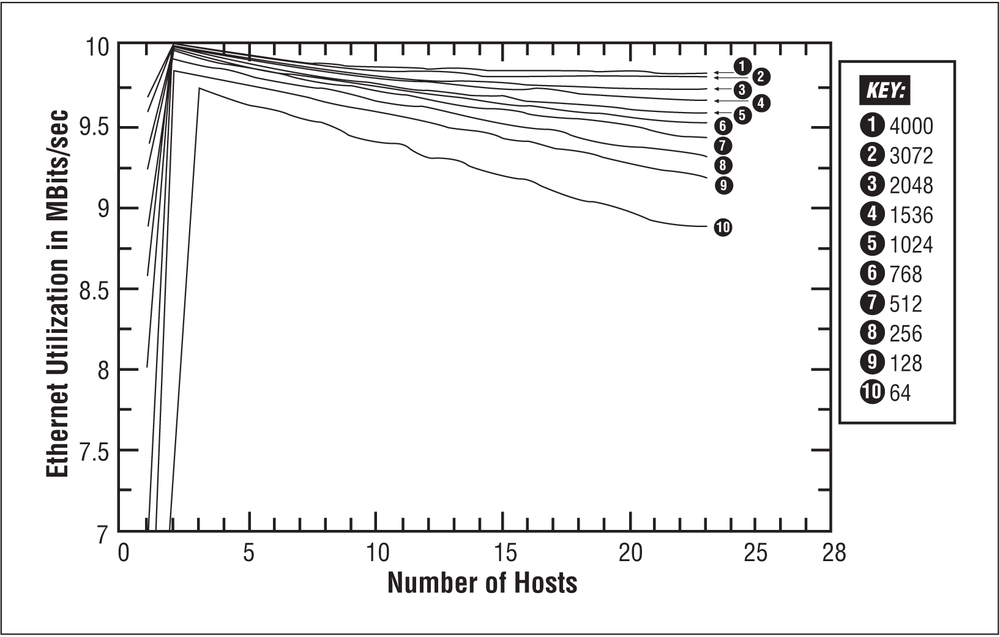
In the Boggs, Mogul, and Kent paper, a population of 24 workstations were programmed to constantly flood a 10 Mb/s Ethernet channel in several experimental trials, each using a different frame size, and some using mixed frame sizes. The results showed that the Ethernet channel was capable of delivering data at very high rates of channel utilization even when the 24 stations were constantly contending for access to the channel. For small frames sent between a few stations, channel utilization was as high as 9 Mb/s, and for large frames utilization was close to the maximum of 10 Mb/s (100% utilization).

With 24 stations running full blast, there was no arbitrary saturation point of 37% utilization (confirming what LAN managers who had been using Ethernet for years already knew). Nor did the system collapse with a number of stations offering a high constant load, which had been another popular myth. Instead, the experiments demonstrated that a half-duplex Ethernet channel could transport high loads of traffic among this set of stations in a stable fashion and without major problems.

Figure 20-1 shows a graph of Ethernet utilization from the Boggs, Mogul, and Kent paper^[69] that illustrates the maximum channel utilization achieved when up to 24 stations were sending frames continuously, using a variety of frame sizes. The frame sizes for each graph are numbered from 1 through 10, and range from 64 bytes (graph number 10) on up to 4,000 bytes (graph number 1). Any frame larger than 1,518 bytes exceeds the maximum allowed in the Ethernet specification, but the larger frame sizes were included in this test to see what would happen when the channel was stress-tested in this way. The graph shows that even when 24 stations were constantly contending for access to the channel, and all stations were sending small (64-byte) frames, channel utilization stayed quite high, at around 9 Mb/s.

The Boggs, Mogul, and Kent paper also provides some guidelines for network design based on their analysis. Two points they made are worth restating here:

Figure 20-1. Ethernet utilization graph

The Boggs, Mogul, and Kent paper noted that some of the theoretical studies that had been made of Ethernet performance were based on simulations that did not appear to accurately model Ethernet behavior. Building an accurate simulator of Ethernet behavior is difficult, because transmissions on an Ethernet are not centrally controlled in any way; instead, they happen more or less randomly, as do collisions.

In 1992, Speros Armyros published a paper showing the results of a new simulator for Ethernet that could accurately duplicate the real-world results reported in the Boggs, Mogul, and Kent paper.^[70] This simulator made it possible to try out some more stress tests of the Ethernet system.

These new tests replicated the results of the Boggs, Mogul and Kent paper for 24 stations. They also showed that under worst-case overload conditions, a single Ethernet channel with over 200 stations continually sending data would behave rather poorly, and access times would rapidly increase. Access time is the time it takes for a station to transmit a packet onto the channel, including any delays caused by collisions and by multiple packets backing up in the station’s buffers due to congestion of the channel.

Further analysis of an Ethernet channel using the improved simulator was published by Mart Molle in 1994.^[71] Molle’s analysis showed that the Ethernet binary exponential backoff (BEB) algorithm was stable under conditions of constant overload on Ethernet channels with station populations under 200. However, once the set of stations increased much beyond 200, the BEB algorithm began to respond poorly. In this situation (under conditions of constant overload), the access time delays encountered when sending packets can become unpredictable, with some packets encountering rather large delays.

Molle also noted that the capture effect, described in Appendix B, can actually improve the performance of an Ethernet channel for short bursts of small packets. However, the capture effect also leads to widely varying response times when trains of long packets briefly capture the channel. Finally, Molle’s paper described a new backoff algorithm that he created to resolve these and other problems, called the Binary Logarithmic Arbitration Method (BLAM). BLAM was never formally adopted by the Ethernet standard, for the reasons explained in Appendix B.

Molle noted that constantly overloaded channels are not a realistic model of real-world usage. What the network users are interested in is response time, which includes the typical delay encountered when transmitting packets. Highly congested channels exhibit very poor response times, which users find unacceptable.

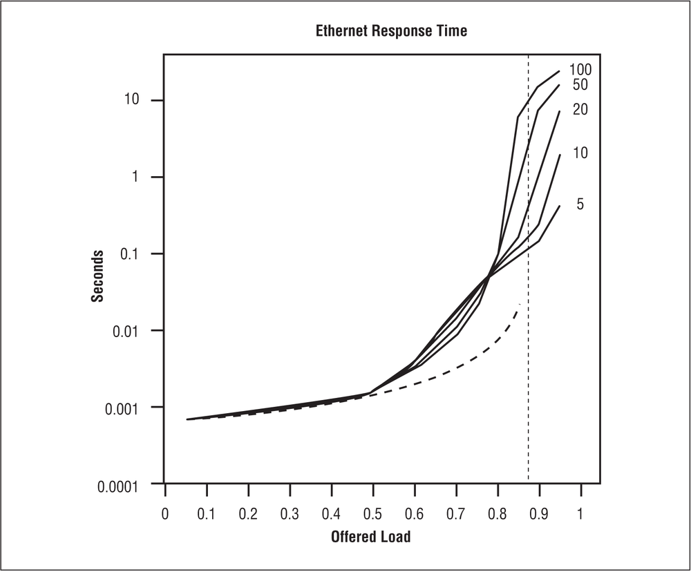
Figure 20-2 shows a graph from Molle’s paper, displaying the effects that channel load and the number of stations (hosts) have on response time.^[72] The chart shows that the average channel response time is good until the channel is seeing a constant load of more than 50%. The region from 50% constant load to about 80% constant load shows increased delays, and above 80% constant load the delays increase rapidly.

Figure 20-2. Ethernet channel access time

Another element is the variation in channel access times, known as jitter. For example, real-time traffic carrying audio information will work best on an uncongested channel that provides rapid response times. Heavily loaded channels can result in excessive delay and jitter, making the audio bursty and difficult to understand. Therefore, excessive jitter will be unacceptable to the users of real-time applications.

The Molle study shows that there are three major operating regimes for an Ethernet half-duplex channel:

The lessons learned in these studies make it clear that users trying to get work done on a constantly overloaded channel will perceive unacceptable delays in their network service. Although constant high network loads may feel like a network “collapse” to the users, the network system itself is in fact still working as designed; it’s just that the load is too high to rapidly accommodate all of the people who wish to use the network.

The delays caused by congestion in communications channels are somewhat like the delays caused by congested highways during commute times. Despite the fact that you are forced to endure long delays due to a traffic overload of commuters, the highway system isn’t broken; it’s just too busy. An overloaded Ethernet channel has the same problem.

Before you set out to measure the network load on a real network, you need to determine what time scale to use. Many network analyzers are set by default to look at the load on an Ethernet averaged over a period of one second. One second may not sound like a long period of time, but a 10 Mb/s Ethernet channel operating flat out can theoretically transmit 14,880 frames in that one second. A Gigabit Ethernet system can send a hundred times that amount, or 1,488,000 frames per second, and a 100 Gigabit system can send 148,800,000 frames per second.

By looking at the load on a network in one-second increments, you can generate a set of data points that can be used to draw a graph of the one-second average loads over time. This graph will rise and fall, depending on the average network traffic seen during the one-second sample period.

The one-second sample time can be useful when looking at the performance of a network port in real time. However, most network systems consist of more than one network segment, and most network managers have better things to do than spend all day watching the traffic loads on Ethernet ports. Management software exists that will automatically create reports of network utilization and store them in a database. These reports are used to create charts that show traffic over the busy hours of a workday, or the entire day, week, or month.

Because the traffic rate on a LAN can vary significantly over time, you really need to look at the average utilization over several time periods to get an idea of the general loads seen on the network. The traffic on most Ethernet ports tends to be bursty, with large, short-lived peaks. Peak network loads can easily go to 80, 90, or 100% measured over a one-second interval without causing any problems for a typical mix of applications.

For an Ethernet system, the minimal set of things you might consider keeping track of include:

The time scales you choose for generating utilization figures are a matter of debate, because no two networks are alike and every site has a different mix of applications and users. Network managers often choose to create baselines of traffic that extend over several time scales. With the baselines stored, they can then compare new daily reports against previous reports to make sure that the Ethernet ports are not staying at high loads during the times that are important to the users.

Most networks are designed in a hierarchy, with access switches connected to core switches using uplink ports. Monitoring those uplink ports is critical, because they are the bottlenecks for your network system. Very high loads on those uplinks that last for significant periods of time during the workday could cause unacceptable delays.

For example, filesystem backups can take a fair amount of time to perform and often place a heavy demand on your network. To ensure that your users have priority access to the network, it’s recommended that you perform backups at night, when the likelihood of user traffic on the network is minimal.

Constant monitoring also provides evidence of overload that can be useful when responding to complaints about network performance. Given the wide variability in application mix, number of users, and so on, it is quite difficult to provide any rules of thumb when it comes to network load. Some network managers report that they regard network traffic as approaching excessive load levels when:

Notice that these recommendations are not based on the three operating regimes derived from Molle’s paper. The three operating regimes that Molle studied are based on one-second average loads on half-duplex shared channels. In the traffic load levels just shown, an eight-hour average utilization that reaches 20% is a heavily smoothed graph, which does not show the short-term peaks. During the business day, we can assume that transient peaks went much higher than 20%. More importantly, we can assume that when the long-term average gets that high, the peak traffic loads may have been lasting for long periods, producing unacceptable response times for the users.

There are many ways to generate graphs and reports of network utilization. Table 20-1 displays some raw data collected with an SNMP-based management program. These samples were collected every 30 minutes for the total number of packets, octets, broadcasts, and multicasts seen on an uplink port.

The average utilization on the channel over the 30-minute period is also collected. Notice that during the 30-minute period from 10:42 to the next sample at 11:12, the average utilization was 25%. This average is high for such a long period of time in the middle of the workday, and network users may have complained about poor response time during this period. A shorter sample time would very likely have shown much higher peak loads lasting for significant periods of time, which could cause poor response times and generate complaints about network performance.

When collecting utilization information, it’s up to you to determine what load levels are acceptable to your users, given the application mix at your site. Note that short-term averages may reach 100% load for a few seconds without generating complaints. Short-term peaks such as this can happen when large file transfers cause high loads for a brief period. For many applications, the users may never notice the short-term high loads. However, if the network is being used for real-time applications, then even relatively short-term loads could cause problems.

When the reports for an Ethernet begin to show a number of high utilization periods, a LAN manager might decide to keep a closer eye on the network. You want to see whether the traffic rates are stable, or if the loads are increasing to the point where they may affect the operation of the network applications being used. The network load can be adjusted by increasing the speed of the Ethernet links, especially the uplinks between switches.

The analytical studies we’ve seen so far were interested in measuring total channel utilization, which includes all application data being sent as well as the framing bits and other overhead it takes to send the data. This is useful if you’re looking at the theoretical bandwidth of an Ethernet channel. On the other hand, most users want to know how much data they can get through the system. This is sometimes referred to as throughput. Note that bandwidth and throughput are different things.

Bandwidth is a measure of the capacity of a link, typically provided in bits per second (bps). The bandwidth of Ethernet channels is rated at 10 million bits per second (10 Mb/s), 100 million bits per second (100 Mb/s), 1 billion bits per second (1 Gb/s), and so on. Throughput is the rate at which usable data can be sent over the channel. While an Ethernet channel may operate at 10 Mb/s, the throughput in terms of usable data will be less due to the number of bits required for framing and other channel overhead.

On an Ethernet channel, it takes a certain number of bits, organized as an Ethernet frame, to carry data from one computer to the other. The Ethernet system also requires an interframe gap between frames, and a frame preamble at the front of each frame. The framing bits, interframe gap, and preamble constitute the necessary overhead required to move data over an Ethernet channel. As you might expect, the smaller the amount of data carried in the frame, the higher the percentage of overhead. Another way of saying this is that frames carrying large amounts of data are the most efficient way to transport data over the Ethernet channel.

Switches provide you with multiple Ethernet channels, and make it possible to upgrade those channels to higher speeds of operation. Each port on a switch can operate at different speeds, as needed, and is capable of delivering the full bandwidth of the channel. Examples of switch configurations are provided in Chapter 19. You can link stacks of switches together, for example, to create larger Ethernet systems.

Today, all computers in the workplace are connected to networks, and everyone in the workplace requires a computer and a network connection. Huge numbers of network applications are in use, ranging from applications that send short text messages to high-definition video. This proliferation of network is leading to a constantly increasing appetite for more bandwidth.

The incredibly rapid growth of the Internet has had a major impact on the traffic flow through local networks. In the past, many computing resources were local to a given site. When major resources were local to a workgroup or to a building, network managers could depend on the 80/20 rule of thumb, which stated that 80% of traffic on a given network system would stay local, and 20% would leave the local area for access to remote resources.

With the growth of Internet-based applications, the 80/20 rule has been inverted. As a result of the Internet and the development of corporate intranets, a large amount of traffic is being exchanged with remote resources. This can place major loads on backbone network systems, as traffic that used to stay local is now being sent over the backbone system to reach the intranet servers and Internet resources and cloud-based services.

Not only is traffic increasing, but multimedia applications that deliver streaming audio and video to the user are in common use. These applications place serious demands on network response time. For example, excessive delay and jitter can cause problems with real-time multimedia applications, leading to breakups in the audio and to jerky response on video displays.

Multimedia applications are currently undergoing rapid evolution. Fortunately, modern multimedia applications are designed for delivery over the Web. These applications typically expect to encounter network congestion and packet loss on the Internet. Therefore, they use sophisticated data compression and buffering techniques and other approaches to reduce the amount of bandwidth they require, and to continue working in the presence of low response times and high rates of jitter. Because of this design, these types of multimedia applications will very likely perform quite well even on heavily loaded campus Ethernets.

About the best advice anyone can give to a network designer is to assume that you will need more bandwidth, and probably sooner than you expect. Network designers should: