
Date representation is a difficult task to complete. It is essential to track dates with financial transactions to glean information such as frequency, patterns, customer information, and due dates; however, unlike numbers, dates cannot be easily graphed via Excel.
In this recipe, you will learn to create a worksheet-based calendar to represent the payment dates visually.
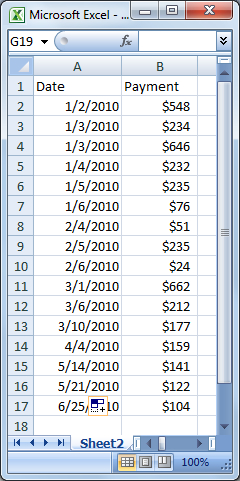
We will start with a worksheet with dates and payment amounts:
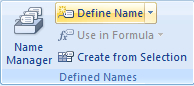
- Select column A, then from the Excel ribbon select Formulas | Define name:
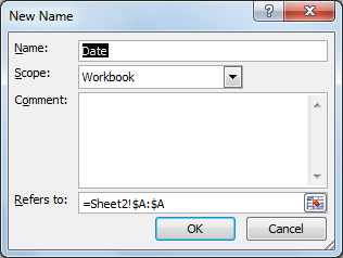
When the name manager opens, the name should already be set as the column title listed in Column A.
- Name the range, Date, and then select OK:
- Repeat the above process with column B, and name the range, Payment.
With the range set to the entire column, we will be able to add new payments to the column as needed.
- Select the next worksheet.
This worksheet will contain the payment calendar.
- Start in column A cell 2, and enter the numbers 1 through 12:
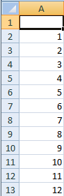
- Repeat the process starting in cell B1 and numbers 1 through 31.
Column A will represent the months within our calendar, and row 1 will represent the day of the week.
- Select B2 and enter the following formula:
=SUM((DAY(Date)=B$1)*(MONTH(Date)=$A2)*(Payment)), then press Ctrl + Shift + Enter.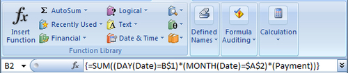
- Select the lower-right corner of cell B2, and drag the cell through column AF.
This will fill the cell formula through the column of 31.
- Click and hold the lower right-hand corner of cell AF2, and drag down to AF13.
This will fill the formula through the rows for the month. You should also notice that the formula has begun to provide data within the calendar. We will now modify the look of the calendar to enhance its visual appearance.
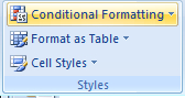
- Select cells B2 through AF13, then from the Home tab on the Excel ribbon, choose Conditional Formatting | New:
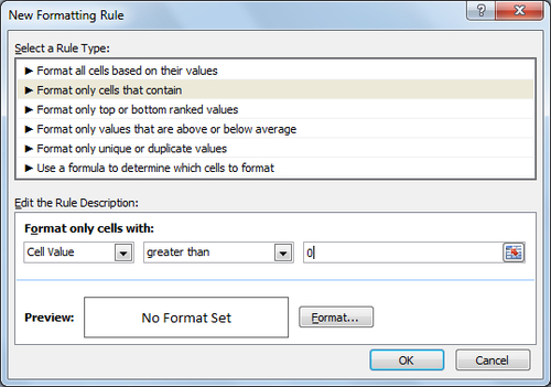
- From the New Formatting Rule window, choose the rule for Format only cells that contain, and enter the rule Cell Value greater than 0:
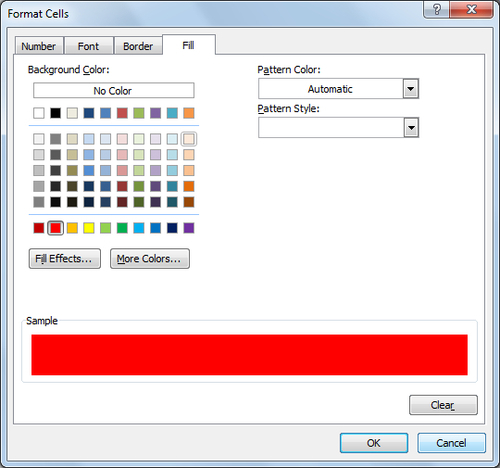
- Choose Format Cells, the Fill tab, change the fill color to red, and then select OK twice:
- With the worksheet cells still selected, change the font color to white.
The graphical calendar displaying payments now displays payments in red:
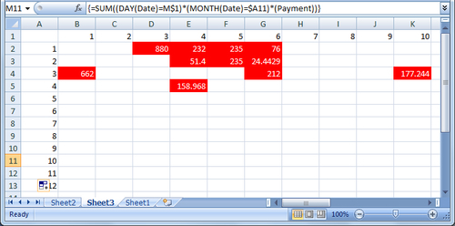
From the graphical calendar, a financial manager can determine the frequency and total of payments as they occur within the calendar. It is clearly evident that from January through April, payments are received within the first six days. The financial manager can now provide investment advice as to the timing of investments and or the ability to float payments as needed to maximize bank interest.
By naming the ranges for the date and payment, we are able to utilize the cell range by name in any sheet within the Excel workbook. This reduces the amount of typing needed to refer to the range. In addition, the range will expand automatically to encompass new payments without needing to update the formulas used.
The formula to SUM the payment on the graphical calendar checks the day and month of each of the payments, and returns the sum of the payment to the corresponding location on the graphical calendar.
Lastly, we utilize conditional formatting to highlight the cells with the payment amounts in red.