

1.2. THE FUNDAMENTAL THEOREM 17
Also notice that we could have found the total area as
A D 2
Z
2
1
.x
2
1/ dx
once we knew the areas above and below the curve were equal. Since it’s not obvious until after
you do the integral, this isn’t all that useful in this case. We will look at a useful version of this
phenomenon later.
Example 1.24 Find the area under y D
1
x
from x D 1 to x D 4.
Solution:
A
4
-1
-1
3
y D
1
x
x D 1
A
Z
4
1
1
x
dx D ln.x/
ˇ
ˇ
ˇ
ˇ
4
1
D ln.4/ ln.1/
D ln.4/ 0
D ln.4/
˙
18 1. INTEGRATION, AREA, AND INITIAL VALUE PROBLEMS
is example pays off on explaining a mystery – why we use e Š 2:71828 : : : as the base of the
“natural” logarithm. It is because the area under y D
1
x
from x D 1 to x D a is ln.a/. is gives
us a method of computing logs, and it shows a place where logarithms arise naturally from the
rest of mathematics. A much better way to choose a base than “we have ten fingers.”
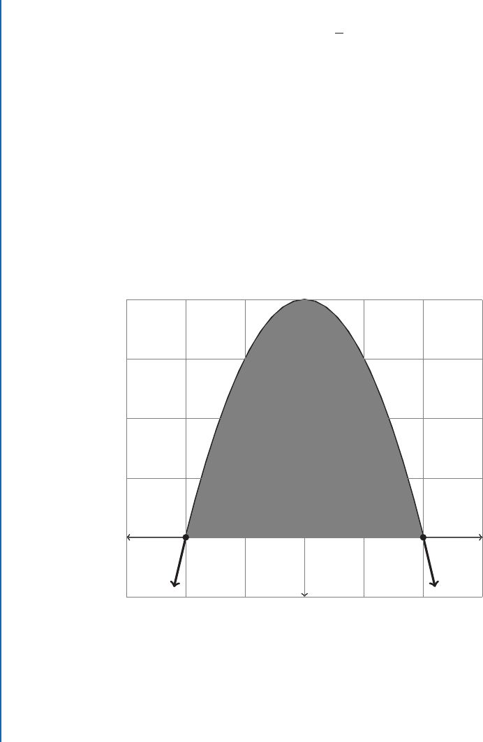
Example 1.25 Find the area bounded by y D 4 x
2
and the x-axis.
Solution:
A
3-3
-1
4
x
D
2 x
D
2
y
D
4
x
2
is problem does not give explicit limits – instead it tells us what the objects bounding the area
are. Since the x-axis is where y D 0, we need to solve 0 D 4 x
2
, which gives us x D ˙2 as the
points at the left and right end of the area. is then gives us a nice everything-above-the-axis
integral.

1.2. THE FUNDAMENTAL THEOREM 19
A D
Z
2
2
4 x
2
dx
D 4x
1
3
x
3
ˇ
ˇ
ˇ
ˇ
2
2
D 4.2/
1
3
8 4.2/ C
1
3
.8/
D 8 C8
8
3
8
3
D 8
2
2
3
D 8
4
3
D
32
3
units
2
˙
Finding the area bounded by two different curves requires solving for those x where
curve 1 D curve 2
in order to find the limits of integration. is will come up a lot in the future. is problem can
be rephrased as curve 1 curve 2 D 0 making it a root finding problem.

20 1. INTEGRATION, AREA, AND INITIAL VALUE PROBLEMS
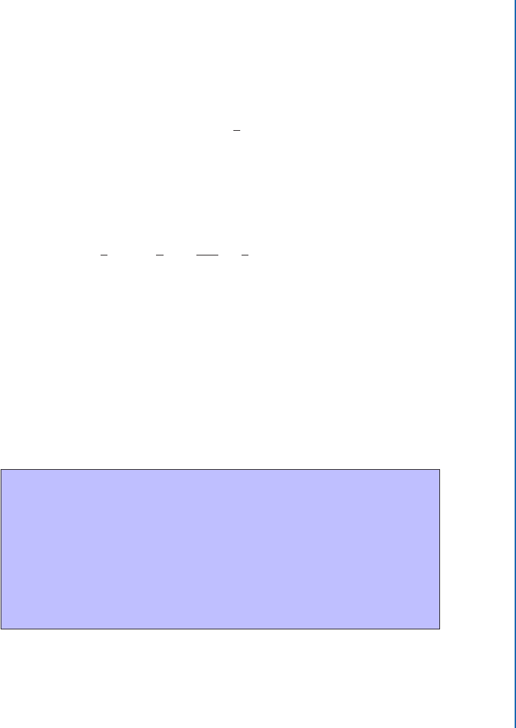
Example 1.26 Find the area bounded by y D x
2
and y D
p
x.
Solution:
2
-1
-1
2
y D x
2
y D
p
x
is one is a little tricky. e picture shows us that if we solve x
2
D
p
x to get the points where
the area begins and ends, then those points are (0,0) and (1,1). e area we want is shown in
dark gray. It is the area under y D
p
x that is not under y D x
2
. If we computed
Z
1
0
p
x dx,
we would get the dark gray area and the light gray area. e light gray area is the area under
y D x
2
. is means the dark gray area is:
Z
1
0
p
x dx
Z
1
0
x
2
dx
Compute
Z
1
0
p
x dx
Z
1
0
x
2
dx D
Z
1
0
x
1=2
x
2
dx
D
2
3
x
3=2
1
3
x
3
ˇ
ˇ
ˇ
ˇ
1
0
D
2
3
1
3
0 C 0
D
1
3
units
2
˙
1.2. THE FUNDAMENTAL THEOREM 21
One thing that might be a little tricky in this example is the slightly odd version of the power
rule:
Z
x
1=2
dx D
2
3
x
3=2
C C
All that is going on is that
1
2
C 1 D
3
2
and
1
3=2
D
2
3
.
To find the area bounded by the curves we first found their intersections and then subtracted
the area under the lower curve from the area under the upper curve. Another point of view
on this is that we integrated the upper curve minus the lower curve. Let’s formulate this as a rule.
Knowledge Box 1.10
Area between two curves
If f .x/ > g.x/ on an interval [a,b], then the area between the
graphs of the two functions on that interval is:
Z
b
a
f .x/ dx
Z
b
a
g.x/ dx D
Z
b
a
.
f .x/ g.x/
/
dx
is rule is handy, but it does leave you with the problem of finding the appropriate intervals.
..................Content has been hidden....................
You can't read the all page of ebook, please click here login for view all page.