
6.3. Fixed Effects as a Latent Variable Model
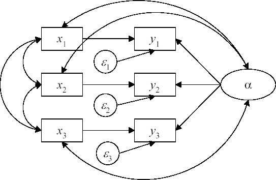
As noted in chapter 2, the basic random effects model is actually a special case of the fixed effects model (Mundlak 1978). The random effects model assumes that αi is uncorrelated with xit, the vector of time-varying covariates. The fixed effects model allows for any correlations between αi and the elements of xit. Figure 6.2 shows a path diagram for a simplified fixed effects model with a single time-varying predictor. The only difference between this diagram and the one in Figure 6.1 is the addition of the curved arrows representing correlations between α and the x variables.
Figure 6.2. Figure 6.2 Path Diagram of a Fixed Effects Model for Three Points in Time
These additional correlations can be easily incorporated into SEM software such as PROC CALIS (Allison and Bollen 1997; Teachman et al. 2001). The default in CALIS is to assume that any latent variables are uncorrelated with all the observed predictor variables. To relax that assumption, we add the COV statement to our previous PROC CALIS program:
PROC CALIS DATA=my.nlsy UCOV AUG;
LINEQS
   anti90=t1 INTERCEPT + b1 pov90 + b2 self90 +b3 black + b4
     hispanic + b5 childage + b6 married + b7 gender + b8 momage +
     b9 momwork + falpha + e1,
   anti92=t2 INTERCEPT + b1 pov92 + b2 self92 +b3 black + b4
     hispanic + b5 childage + b6 married + b7 gender + b8 momage +
     b9 momwork + falpha + e2,
anti94=t3 INTERCEPT + b1 pov94 + b2 self94 +b3 black + b4
hispanic + b5 childage + b6 married + b7 gender + b8 momage +
b9 momwork + falpha + e3;
STD
falpha e1 e2 e3 = s1 s2 s2 s2;
COV
falpha*pov90 pov92 pov94 self90 self92 self94 = c:;
RUN;The COV statement allows a covariance (correlation) between FALPHA and each of the six variables representing the two time-varying explanatory variables, SELF and POV. The C: at the end of the statement says to name these covariances C1, C2, ..., C6. Note that a correlation cannot be allowed between FALPHA and any time-invariant predictors such as GENDER or MARRIED. Attempting to do so results in what is called an underidentified model, which may produce the following warning message in PROC CALIS:
NOTE: Covariance matrix for the estimates is not full rank.

NOTE: The variance of some parameter estimates is zero or some
      parameter estimates are linearly related to other parameter
      estimates as shown in the following equations:
The coefficient estimates and associated statistics for the fixed effects model are shown in Output 6.3. Only one equation is displayed because the other two are identical except for the intercept. Looking first at the coefficients for SELF and POV, we see that they are identical to the fixed effects estimates in Output 2.10, estimated with PROC GLM, and Output 2.21, estimated with PROC MIXED. The standard errors and t-statistics are also identical. Like the PROC MIXED results in Output 2.21, we also get estimates for the time-invariant variables. However, the estimates and test statistics in Output 6.3 for these variables are quite different from the estimates and test statistics in Output 2.21. For example, the coefficient for MOMWORK in Output 6.3 is clearly statistically significant, but is just as clearly not significant in Output 2.21. Why the difference? One clue is that when the mean scores for poverty and self-esteem (MPOV and MSELF) are removed from the model in Output 2.21, the results for the time-invariant variables, although not identical to those in Output 6.3, are quite close and certainly in qualitative agreement. This makes sense, because the CALIS model has no comparable variables to the mean scores (and, so far as I can tell, no way to include them).

|
| Variances of Exogenous Variables | ||||
|---|---|---|---|---|
| Variable | Parameter | Estimate | Standard Error | tValue |
| falpha | s1 | 1.30190 | 0.09751 | 13.35 |
| e1 | s2 | 0.99244 | 0.04121 | 24.08 |
| e2 | s2 | 0.99244 | 0.04121 | 24.08 |
| e3 | s2 | 0.99244 | 0.04121 | 24.08 |
Now that we have both a fixed effects and random effects version of our model in PROC CALIS, it is a simple matter to produce a likelihood-ratio statistic to compare them. For each model, the output contains a chi-square statistic and associated degrees of freedom. This statistic compares the overall fit of the model to a saturated model that perfectly reproduces the covariance matrix for all the variables. For the random effects model of Output 6.1, the chi-square is 84.4180 with 34 degrees of freedom. For the fixed effects model of Output 6.3, it's 66.4505 with 28 degrees of freedom. The difference between the two is a chi-square of 18.0305 and 6 degrees of freedom. The six degrees of freedom correspond to the six additional correlations that are allowed under the fixed effects model. The p-value for this chi-square is .006, indicating that we should reject the random effects model in favor of the fixed effects model. This is the same conclusion that we reached in chapter 2 using either the Hausman test produced by PROC TSCSREG or the tests of equality for coefficients of the mean and centered scores. (Both of those tests had 2 degrees of freedom.) From a theoretical point of view, however, the likelihood ratio test computed here is more elegant and might have better statistical properties. The Hausman test, for example, could have negative values for some data configurations, but this not possible for the likelihood ratio test.