
1.2. The Paired-Comparisons t-Test as a Fixed Effects Method
Perhaps the simplest design that meets these two requirements is a before-after study. Suppose, for example, that 100 people volunteer to participate in a weight loss program. They all get weighed when they enter the study, producing the variable W1. All 100 people are then given a new medication believed to facilitate weight loss. After two months on this medication, they are weighed again, producing the variable W2. So we have measurements of weight on two occasions for each participant. The participants are off the medication for the first measurement and are on the medication for the second.
How should such data be analyzed? Before answering that question, let's first concede that this is not an ideal study design, most importantly because there is no control group of people who don't receive the medication at either time. Nevertheless, the application of fixed effects methods has all the virtues that I claimed above. The objective here is to test the null hypothesis that mean weight at time 1 is the same as mean weight at time 2, against the alternative that mean weight is lower at time 2. In this case, an easily applied fixed effects method is one that is taught in most introductory statistics courses under the name of paired-comparisons t-test or paired-differences t-test. The steps are:
The third step is accomplished by dividing ![]() by its estimated standard error
by its estimated standard error ![]() , where s is the sample standard deviation of D, and n is the sample size. The resulting test statistic has a t distribution with n – 1 degrees of freedom under the null hypothesis (assuming that D is normally distributed).
, where s is the sample standard deviation of D, and n is the sample size. The resulting test statistic has a t distribution with n – 1 degrees of freedom under the null hypothesis (assuming that D is normally distributed).
If ![]() is significantly less than 0, what can we conclude? Well, we can't be sure that the medication caused the weight loss, because it's possible that something else happened to these people between time 1 and time 2. However, we can be sure that the difference in average weight between the two time points is not explainable by stable characteristics of the people in the study. In other words, we can be quite confident that the weight loss was not produced by changes in race, gender, parental wealth, or intelligence.
is significantly less than 0, what can we conclude? Well, we can't be sure that the medication caused the weight loss, because it's possible that something else happened to these people between time 1 and time 2. However, we can be sure that the difference in average weight between the two time points is not explainable by stable characteristics of the people in the study. In other words, we can be quite confident that the weight loss was not produced by changes in race, gender, parental wealth, or intelligence.
While this conclusion may seem obvious, it's helpful to consider a mathematical formulation as a way of introducing some of the ideas that underlie the more complicated models considered later. Let
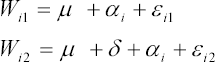
where Wi1 is the weight of person i at time 1, and similarly Wi2 is the weight at time 2. In this model, μ is the baseline average weight, and δ denotes the change in the average from time 1 to time 2. The disturbance terms εi1 and εi2 represent random variation that is specific to a particular individual at a particular point in time. As in other linear models, one might assume that εi1 and εi2 each have an expected value of 0. The term αi represents all the person-specific variation that is stable over time. Thus αi can be thought to include the effects of such variables as race, gender, parental wealth, and intelligence.
When we form the difference score, we get
which shows that both the baseline mean μ and the stable individual variation αi disappear when we compute difference scores. Therefore, the stable individual differences can have no effect on our conclusions, even if αi is correlated with εi1 or εi2.
The essence of a fixed effects method is captured by saying that each individual serves as his or her own control. That is accomplished by making comparisons within individuals (hence the need for at least two measurements), and then averaging those differences across all the individuals in the sample. How this is accomplished depends greatly on the characteristics of the data and the design of the study.